

Introduction of the 2-Body Problem
In the last orbital dynamics post I introduced the n-body problem and how there is no general analytic solution. There is a general analytic solution for a simplified version of this problem called the 2 body problem, and that’s what this post, and the next several, will be about. In this simplified version, we are only concerned with 2 bodies acting on each other gravitationally. More specifically, we are interested in cases where one body is much larger than the other. An example of this is a spacecraft orbiting the Earth. Both exert a force on the other, but because the Earth is much more massive than the spacecraft, we can ignore the forces acting on it. Another example of an object orbiting around a much larger object, is the earth orbiting around the sun.
While this is a restricted set, it is applicable to many different objects of interest. We can simplify our analysis some more if we don’t consider both objects to be moving, but instead consider the larger object fixed and the smaller objects moving relative to the larger. This simplifies our analysis and means we only need to keep track of 6 states instead of 12.
Integrals of the 2-Body Problem
The equation of motion is,


Because we are only tracking one body relative to the second we only need this one equation of motion instead of two coupled together. Now, we can see through inspection that it’s nonlinear, and nonlinear equations are hard to integrate analytically. Luckily there are some clever tricks we can use to turn this equation into something we can integrate, and through those processes we are going to uncover important insights into the bodies orbit.
Note:If you have Batton’s Introduction to Astrodynamics I’m covering section 3.3. If you have Dover’s Fundamentals of Astrodynamcis I’m covering sections 1.4 – 1.8. My post will be much more similar to Batton but I recognize Dover is a much cheaper, although less in depth, alternative.
Angular Momentum
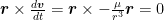
First lets left cross multiply the equation of motion with the position vector


Note: A bold character in an equation is a vector and an unbolded character is a scalar.
Note: I’m going to walk through this derivation a little more then the rest of them but that doesn’t mean that you shouldn’t go into the nitty gritty on your own. I’ll be skipping steps to ensure this post is not super long but I encourage you to have a notepad and pen with you to work through unstated steps. This is the best way to ensure you understand whats going on.

Now in the above equation we can see we are crossing a vector with a scaled version of itself. Any vector cross a scaled version of itself is 0. Now lets take a moment to visit the product rule for vector derivatives which says

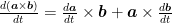
Now if we replace the a and b in the above equation with r and v respectively and remember that both the derivative of r is v and and that a vector crossed with itself is 0 we can obtain the following relationship.


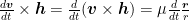
Combining this relationship with the fact we know the position cross the governing equation is zero we get the following relationship.


In this form it’s trivial to integrate over time and we get


h is a vector representing massless angular momentum. From this we can easily see that angular momentum is constant and that all the motion takes place in a single plane where


Eccentricity
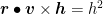
Now lets right multiply the governing equation with the angular momentum vector, which is a constant. When we do that we get the following relationship

Like before this is able to be integrated and we obtain the following equation


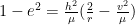
The e vector in the above is the eccentricity vector. The magnitude of the eccentricity vector gives us the eccentricity of the orbit which is a measure of how squished vs circular the orbit is.
Semilatus Rectum
Now that we have derived the eccentricity vector, lets take its dot product with itself.


Now, that’s an unwieldy expression so lets evaluate it in chunks. First,


The second chunk,

Now let’s put it all back together again

Now that its all back together, let’s pluck out the first factor and call it the parameter or semi-latus rectum (feel free to let your inner 12 year old giggle)


If you’re keeping track of the units, which you should be, the semi latus rectum has units of length. The second factor that we will pull out is

Now, to some of you, the above statement looks somewhat familiar. Lets reorganize it into the following


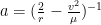
Now that its rearranged it might be easier to see. The first term is the kinetic energy, and the second is the potential energy. By adding them together we get the Total energy which is always constant. By rearranging the terms one more time we get what is known as the energy integral or the vis-viva integral, reproduced below.


It is easy to see the relationship between p, a and e in the following equation


If we know two of those 3 elements we can determine the path that the orbiting object will take. In order to determine it’s location on that path we will need to know one more piece of information, the time of perricenter passage.
Time of Perricenter Passage
The point in the orbit where the two bodies come closest is called the pericenter. The time that the body we are observing goes through the pericenter is called the time of pericenter passage and is referred to by its symbol τ. If we know both τ and the current time we can determine where on the orbit the body currently is.
Now this constant comes from integrating the following equation which relates true anomaly, f, to time.

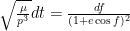
The true anomaly is the angle between the position vector and the eccentricity vector we found earlier in the post. Trough observation you can see that the above equation does not lend itself to being integrated easily. Trying to integrate the above equation drove many important advances in mathematics that will be covered in future posts.
Takeaway and next weeks post
This was a long and very math filled post. If you made it this far give yourself a pat on the back. Next weeks post will be focused on giving you a more intuitive understanding of the concepts discussed here by explaining their geometric significance. It’ll have a lot of graphics and, if I get it working, an interactive component. If you want to receive the weekly Gereshes blog post directly to your email every Monday morning you can sign up for the newsletter here!
If you can’t wait for next weeks post and want some more Gereshes I suggest