

Balancing a Marble
Imagine you had a marble and you wanted to put it at the point between the Earth and the Moon where the force of gravity was equal from both. The two forces would cancel out, and the marble would remain in that location forever. If the sun and the earth were not moving, there would only be one of these points, but because the Earth and the Moon are both orbiting around a common barycenter there are 5 of these points that always remain in constant relative positions to the main bodies. They are called Lagrange points, after the man who discovered them Joseph-Louis Lagrange, and are some of the most interesting points in the 3-body problem.

Note: The Lagrange points have a numbering scheme that isn’t always consistent. Generally L1 is between the two bodies, L2 is the one near the secondary (smaller) body, L3 is the one near the primary (larger) body, and L4/L5 are at the +Y/-Y points of the triangles respectively.
Note: this is an ongoing series on the CR3BP. If you want to get ahead on your own these are some good books on the material and astrodynamics in general (Book 1, Book 2, Book 3, Book 4).
Finding Equilibrium
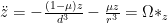
At these Lagrange points, all the forces acting on the particles will be equal and cancel each-other out, which is were they get the name equilibrium points from. A more rigorous definition of a Lagrange point is one where all time derivatives of position are zero in the rotating reference frame. That means velocity and acceleration are both zero. The equations of motion that we found in a past post are as follows.
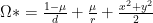
where Ω*, the pseudo potential is defined as
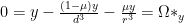
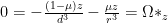
By applying our rule, that all accelerations and velocities must be zero, we get the following
Through inspection we can see that the last equation requires z=0 to be satisfied, so we can ignore that one.


Collinear Lagrange Points
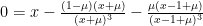
Again, through inspection, we can see that y=0 will also satisfy our equations, so, for now, lets set it to 0. This leaves us with a single equation
if Y and Y are zero than that simplifies our d and r terms to the following
We should now place those into our equations, but don’t cancel out any like terms just yet
From the fact that the above equation is third order, it should have 3 roots, and those three roots will be the positions of 3 Lagrange points. Because we set Y=0 to find these points, we call these Lagrange points the collinear Lagrange points. Now for some bad news. We don’t have simple analytic expressions for the positions of the collinear Lagrange points, but we can find them out through numerical methods. The most popular method for finding them is Newton’s Method which I covered here. You should code up your own Newton’s method to find them. If you want to check your work, in the sun-earth system you should find the following


- L1 – X= 0.609 , Y=0
- L2 – X= 1.260 , Y=0
- L3 – X=-1.042 , Y=0

Equilateral Lagrange Points
Next, we’re going to go to the two Lagrange points where Y is not 0. These are called the equilateral Lagrange points because they lie on the points of an equilateral triangles. The primary and secondary bodies lie on the other points of the equilateral triangles. A nice geometric proof of this can be found here. The x and y coordinates of the equilateral Lagrange points do have nice analytic expressions for them which are


Changing μ
What if we change the mass ratio between the two bodes? The Lagrange points qualitative shapes stay the same, but the actual positions do move. Also, now that the primary body is only 9 times larger than the secondary body, we can see that the primary body is not stationary. Both bodies orbit around the barycenter. Usually in systems like the Sun-Earth or Earth-Moon, the primary is so massive that the barycenter is almost directly on top of the primary’s center of mass.

Questions about Lagrange points
We now have 5 equilibrium points. Once you find equilibrium points in any dynamic system your next question should be “Are they stable?” But to answer that I’ll be creating another blog post. It’s then that I’ll also show you an aspect of the CR3BP that is not possible in a two-body problem. Orbits not around any body, but instead around empty space. Here’s a little teaser

The Lagrange points are where a lot of really cool effects take place, and because smooth space around equilibrium points is linear, we can analyze them in great detail. Now that we have found the Lagrange points, our adventures in the unintuitive and lovely world of the CR3BP can truly begin.
Want more Gereshes
If you want to receive the weekly Gereshes blog post directly to your email every Monday morning, you can sign up for the newsletter here! Don’t want another email? That’s ok, Gereshes also has a twitter account and subreddit!