Dynamics of the 3-Body Problem

Recap

In the last post we introduced the 3-body problem along with some constraints that turned it into the circular restricted 3-Body Problem (CR3BP). In the beginning of that post, I had a GIF that traced out a trajectory in the Earth-Moon system. In this post, we will derive the equations of motion for the Circular Restricted 3-Body Problem (CR3BP) which were used to generate that GIF as well as some numerical techniques for numerically simulating the system.

Note: this is an ongoing series on the CR3BP. If you want to get ahead on your own these are some good books on the material and astrodynamics in general (Book 1, Book 2, Book 3, Book 4).

Rules of the Game

It’s always good to remind ourselves of the rules of our problem and what the problem is.

The rules of the classical 3-Body problem are simple

We have three bodies
They are all point sources and we know their masses
They only interact gravitationally

With the CR3BP we introduced two new rules

The masses of the first two objects are much greater than the mass of the third. M1,M2 >> M3
The two primary bodys move about the barycenter in circles (orbits with zero eccentricity). e1 & e2 = 0

The problem is, given complete state information (instantaneous position, velocity, time) can we predict the third bodies motion into the future?

FBD

Let’s begin with a free body diagram

Inertial Reference Frame

Now that we’ve drawn a basic free body diagram, let’s draw a second with the origin at the barycenter. One axis is the line passing through both planets, the third is in the direction of angular momentum of the system, and the second completes a right hand triad. I’ve drawn these new axis in gray and without a bolded x and y. The z-axis for both is coming out of the page, and the rotational rate of the reference frame is drawn in green.

Rotating Reference Frame

You’l notice that as the planets rotate around the barycenter, the x-axis will change. It will rotate around with the planets at a constant rate. This isn’t an inertial reference frame, but a rotating reference frame. Forces, behave a bit differently here (You’ve experienced this reference frame if you’ve ever been in a car that went around a corner too fast), but we’ll get to that soon. For now, just know that this rotating reference frame will help revel structure hidden in the CR3BP.

Characteristic values

Let’s take a look at things that stay constant in the CR3BP. First we have the distance between the two primaries, lets label this quantity l*.

Rotating Reference Frame with L*

Next we have the sum of the masses of the primary m*. For convenience let’s define a mass ratio of the second body’s mass to m*

$\mu=\frac{m_2}{m^*}=\frac{m_2}{m_1+m_2}$

Note, this μ is different than the μ in the two body problem.

We can use the universal gravitational constant to define a characteristic time

$t* = \sqrt{\frac{l^{*3}}{\tilde{G}m^*}}$

From the FBD in the rotating reference frame, we have vectors going from the barycenter, primary body, and secondary body, to the spacecraft. We divide each of these by the characteristic length to non-dimensionalize these vectors.

$\vec{\rho}=\frac{\vec{r}_3}{l*}=x\hat{x}+y\hat{y}+z\hat{z}$

$\vec{d}=\frac{\vec{r}_{13}}{l*}=x+\mu\hat{x}+y\hat{y}+z\hat{z}$

$\vec{r}=\frac{\vec{r}_{23}}{l*}=x-1+\mu\hat{x}+y\hat{y}+z\hat{z}$

We can also non-dimensionalize time using our characteristic time

$\tau = \frac{t}{t*}$

Why do we want to non-dimensionalize our quantities?

Simulations run better
Helps generalize our results between different systems

Kinematics of Motion

We’re in a rotating reference frame, so we now have to deal with fictitious forces (link) when we take derivatives. We can appeal to the kinematic transport theorem here to get expressions for these new fictitious forces in the rotating frame.

$^I\frac{dp}{dt}^{\omega} = ^I\frac{dp}{dt} + \omega \times p$

If we do this a second time we get the following kinematics of motion in our rotating reference frame.

$^I\ddot{\vec{\rho}}= (\ddot{x}-2y-x)\hat{x}+(\ddot{y}+2\dot{x}-y)\hat{y}+\ddot{z}\hat{z}$

What this equation does is connect the any forces in the inertial reference frame to motion in the rotating reference frame by introducing the required fictions forces. For now you are going to have to accept this very handwavey section on kinematics. This post is not long enough to go over kinematics and rotating reference frames in detail but I plan on giving each of them their own “introduction to” posts. I do not have planned release dates for them yet.

Newton

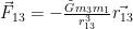
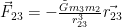
Now let’s use Newtons law of gravitational attraction to find the forces on the particle. Because we’ve limited ourselves to gravitational forces, we only have two. The force on the body from the first and second body respectively.

$\vec{F}_{13} =-\frac{\tilde{G}m_3m_1}{r_{13}^3} \vec{r_{13}}$

$\vec{F}_{23} =-\frac{\tilde{G}m_3m_2}{r_{23}^3} \vec{r_{23}}$

Combining those with newtons second law, we get the acceleration

$m_3 \vec{\ddot{r_3}} = \frac{-Gm_1m_3\vec{r_{13}}}{|r_{13}|^3}-\frac{Gm_2m_3\vec{r_{23}}}{|r_{23} |^3}$

Using our characteristic quantities from earlier , we can once again non-dimensionalize these forces

$\ddot{\vec{\rho}}=-\frac{1-\mu}{d^3}\vec{d}- \frac{\mu}{r^3}\vec{3}$

We now have the non-dimensional inertial acceleration, as well as an equation relating inertial acceleration to movement in the rotating reference frame from the kinematics section. Let’s combine both of them into the equations of motion for the rotating reference frame.

$\ddot{x}-2\dot{y}-x = -\frac{(1-\mu)(x+\mu)}{d^3}- \frac{\mu(x-1+\mu)}{r^3}$

$\ddot{y}+2\dot{x}-y = -\frac{(1-\mu)y}{d^3}- \frac{\mu y}{r^3}$

$\ddot{z} = -\frac{(1-\mu)z}{d^3}- \frac{\mu z}{r^3}$

Observations of the Equations of Motion

Let’s take a few moments to look at the above equations of motion and make some observations. The first is that they are nonlinear. This is due to the cubed d and r in the denominator. Next we should note that they are coupled. The X and Y equations of motion have a y and x velocity in them respectively. This means that we cannot separate and solve them individually, we have to solve them together. The z equation of motion is (relatively) uncoupled from the other two. This means that if we want to only simulate planar motion it will always be in the x-y axis as exciting one will excite the other.

Gravitational Potential

Because we are dealing with gravity, which we know is conservative, we know that the force at any location can be written as the gradient of some potential, Ω

$\vec{F}=-\nabla \Omega$

Because we’re in the rotating frame, lets define some pseudo-potential Ω*.

$\Omega* = \frac{1-\mu}{d}+\frac{\mu}{r}+\frac{x^2+y^2}{2}$

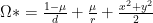
Negative Pseudo-Potential of the Earth-Moon System

This can be found a number of ways, but why do we want this pseudo-potential? Because it will provide a compact way of writing equations in the future. If we want to signify the x derivative of the pseudo-potential we would write

$\Omega_x* = x - \frac{(1-\mu)(x+\mu)}{d^3}-\frac{\mu(x-1+\mu)}{r^3}$

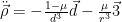
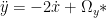
This compact notation lets us rewrite the equations of motion as

$\ddot{x}=2\dot{y}+\Omega_x*$

$\ddot{y}=-2\dot{x}+\Omega_y*$

$\ddot{z}=\Omega_z*$

Note: this is an ongoing series on the CR3BP. If you want to get ahead on your own these are some good books on the material and astrodynamics in general (Book 1, Book 2, Book 3, Book 4).

Want more Gerehses …

If you want to receive the weekly Gereshes blog post directly to your email every Monday morning, you can sign up for the newsletter here! Don’t want another email? That’s ok, Gereshes also has a twitter account and subreddit!
If you can’t wait for next weeks post and want some more Gereshes I suggest

An Introduction to Error

Asteroid Wars – Part 1

My Undergraduate EDC