An Introduction to Error

Good Enough

Numerical methods are always concerned with the term “good enough”. Whether you are using a finite difference to approximate a derivative, or Newtons method to find the roots of a function, we rarely get an exact answer. Usually, our answer is different from the truth by some amount. We generally don’t know what our error is, but we can quantify its likely magnitude, and can generally tweak parameters in our method to make it smaller. As we tweak our method, our error hopefully decreases and we converge to the truth.

Finite Concrete

Let’s return to finite differences. I won’t go over the derivations again here, but in that post, we derived that the error term associated with the finite difference is a function of h, the step size. If we were using a forward difference, the error was just a function of h, but when we analyzed a central difference it was a function of h squared. Let’s explore what this means through a real example.

Let’s say we have a function

$f(x) = sin(x)$

It’s a simple function whose derivative is known exactly as

$f'(x) = cos(x)$

Evaluating at the point π/4 we know the derivative exactly.

$f'(\frac{\pi}{4}) = \frac{\sqrt{2}}{2}$

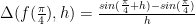
Let’s setup two new functions to find the derivative at this point using a forward and central difference respectively so that they are now only functions of h.

$\Delta (f(\frac{\pi}{4}),h) = \frac{sin(\frac{\pi}{4}+h)-sin(\frac{\pi}{4})}{h}$

$\delta (f(\frac{\pi}{4}),h) = \frac{sin(\frac{\pi}{4}+h)-sin(\frac{\pi}{4}-h)}{2h}$

Now, for this problem we know what we should get so we can evaluate the error in our functions numerically by sweeping though different h’s

Note: be aware of the x axis. the h get’s smaller the farther right we go

We can see that as we make h small our error gets smaller. With the forward difference, the error looks like a downward sloping line so we call it linear. If we halve our h, our error gets cut in half. With the central difference it looks like one side of a parabola, so we call it quadratic. If we halve our h, our error is now a quarter of its former value. It appears that as we get closer to the end of the region we see both converge at the same point, but we’re dealing with extremely small numbers so let’s convert this plot to a log-log scale

Now we can see that the central difference continues to provide better estimates of the derivative and gets better faster as we would expect from the theory. When plotted on a log-log scale both appear as lines, but the slope would now determine the rate of convergence. The steeper the slope, the faster the convergence. Can we continue this trend of getting better approximations for the slope by decreasing h? let’s find out

Going to Machine Precision

Our theory says we should be able to keep getting better approximations by decreasing h, but in both sets, there appears to be a best value of h. What’s more interesting is that it appears that as we keep making h smaller, both approximations, appear to have the same error. What’s happening?

The Noise floor

Unfortunately, computers are not perfect machines. Like us, they have all sorts of flaws. They cant deal with infinitely long numbers so they just cut them off at a certain point to make them finitely long. They round numbers so they can store them in their memory. I plan on turning machine representations of numbers and sources of error into a completely new post so I won’t explain them here. Long story short, computers make mistakes all the time, but we often only see them when we work with two numbers that have a really large difference between them. If you want an introduction to the errors computers generally make this book would be a good starting point.

Defining Error

So we have expanded on the error in a finite difference, but let’s take a moment to define error more generally. If we were to ask people on the street, how they define error, they would probably respond with whether something is right or wrong. With the equation

$3x+9=0$

we can easily see that x is equal to -3. Any other number would be wrong, but let’s say we gave this problem on a math quiz. Student A gives an answer of -4, and student B gives an answer of -7. Both of them are wrong, but which of them is more correct? Instinctively we would say student A.

Student A is only off b 1

Student B is off by 4

4 is greater than 1 so therefore student A is more correct. Here, we defined error as

$Error = -3 - (answer)$

We can rewrite this in a more mathematical way as

$Error = Actual - Answer = Reference - Actual$

Then the one with the lowest error is the most right. But what if we have two more students, C and D, who answer -3 and 4 respectively.

Student C is off by 0 and student D is off by -7. By our old method, now student D has the lowest number and would be the most right. This doesn’t make sense as student C is actually correct. Let’s define a new metric for error that measures the magnitude of the difference instead of the difference itself and call it Error2.

$Error2 = \sqrt{(Reference - Actual)^2}$

Now with the above error function defined, the students, A B C D, get the following errors respectively, 1 4 0 7. This means we can use our original test of using the minimum value to find whose most right. The function we called Error2 is commonly known as the Root Mean Square Error (RMSE).

Why did I Define a Different Error at First?

Home

The RMSE definition of error allows us to easily rank how far away a set of numbers are from a desired value, but in creating it we lose an important piece of information. We lose which direction the error is in. An answer of -4 and -2 would be equivalent using RMSE. Let’s say you are now driving on a north-south road and you’re trying to navigate home. It’s really dark, there’s a new moon, and you live in the country so it’s really hard to see your house so you turn on your GPS. If it uses RMSE to calculate your distance from home you would learn that you are two miles away from your house, but you wouldn’t know whether you needed to drive north or south of your current location. I’ve illustrated this with the figure to the right, with the false home drawn in blue an equal distance away from your real home.

If on the other hand, your GPS used our original error definition you would be able to figure it out. If it gave you a positive number, you would need to drive north, while if it gave you a negative number, you would need to drive south.

Your decision is being driven (pun very much intended) by the sign of the error. In control theory and most numerical methods, the updates to iterative equations are driven by the error. In Newtons method, for example, the size of the update step we take is proportional to the magnitude of the error, while it’s direction is driven by the sign of the error.

Are these the only two ways to define error?

No!

You can define an error function in any way that suits your problem. If you want to make certain things count more you can define a weighted error function. If you googled “error function” Wikipedia, probably your first result would define the error function as

$erf(x)=\frac{1}{\sqrt{\pi}}\int_{-x}^{x}e^{-t^2}dt$

This error function has an important connection to probabilities that’s beyond the scope of this post.

Most, if not all, machine learning techniques are just iterative ways to minimize a certain error function under some set of constraints. Error functions are the driving forces behind machine learning, and choosing the wrong error function can make even the most advanced machine learning techniques worthless. From simple linear regression developed by Gauss/Legendre* to modern neural nets, if you dig into them deep enough you’ll find an error function.

Note: it appears that Legendre was first to publish, but its usually attributed to Gauss as they were only a few years apart.

Quick Recap

Ok, so this post was a bit of a roller coaster. Take a deep breath. We started out on error analysis of a numerical method and ended up with error functions driving machine learning.

Isn’t error awesome?

(wow I just realized I’ve turned into that math teacher whose excited about math)

This post originally began life as an intro on convergence a month ago. I wanted to tie error analysis to convergence analysis, but then I realized I had already typed out a full post without mentioning convergence. Convergence has gone back into the idea bin and I’ll give it another try again soon.

Note: If you have gotten through this whole post and are wondering when I’ll get to human error, I wont be getting to that in this post. However if you’re interested in reducing human error I recommend this book.

Note 2: Error is such an expansive topic that pops up in every discipline so it can have quite a few different meanings. This is not an all encompassing post, and you will find new and different ways to define error. Hopefully this post has whetted your appetite to go and explore other types of error and how it holds us back and propels us forward!

Want more Gerehses …

If you want to receive the weekly Gereshes blog post directly to your email every Monday morning, you can sign up for the newsletter here! Don’t want another email? That’s ok, Gereshes also has a twitter account and subreddit!

If you can’t wait for next weeks post and want some more Gereshes I suggest

The Math behind swinging a swing

Newton’s Method

My Undergraduate EDC