An Introduction to Gradient Descent

Bumpy Terrain

Imagine you are halfway up a mountain. Half an hour ago you decided to start bushwhacking and now you’re completely turned around and lost. What’s worse is that you’ve also lost your map and compass. It’s getting late and you need to get back to your home at the foot of the mountain. What do you do?

Well, you see the ground climb up to what looks like it’s peak in one direction, and you decide to go in the opposite direction. As you walk, the downward slope you are on begins to turn a little, and you turn to follow it. You always keep walking in the direction of the steepest downward slope.

This is, in a nutshell, gradient descent.

From Words to Math

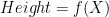
In the problem stated above, we have some value that we want to minimize. In this case, it’s our height on the mountain. The height depends on our location, so in math speak we can write out that height is a function of our location, X.

$Height = f(X)$

For compactness sake, lets call out height z and our location can be given as a vector of coordinates in the x,y plane denoted capital X. We can now write our above function in the form

$z=f(X)$

$X=[x,y]'$

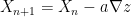
We want to take a step in a direction that makes z as small as possible, we do this by using the gradient operator, ∇

$X_{n+1}=X_n - \nabla z$

If we return to our earlier analogy about walking down a mountain, the longer our legs the larger the more ground we cover with each step. We can introduce this step size scaling as some constant a

$X_{n+1}=X_n-a\nabla z$

Valley Folk

image our home was now located in a valley that can be defined with the following function

$Z(x,y) = x^2 + 2x^2y^2 + 5y^2$

Our home is located in the deepest part of the valley at position (0,0). If we start at a random (x,y) coordinate we can use gradient descent to get home. Our update equations for x and y would be the following

$x_{n+1}=x_n - a(2x_n+4x_ny_n^2),$

$y_{n+1}=y_n - a(10y_n+4x_n^2y_n).$

Let’s see how that evolves

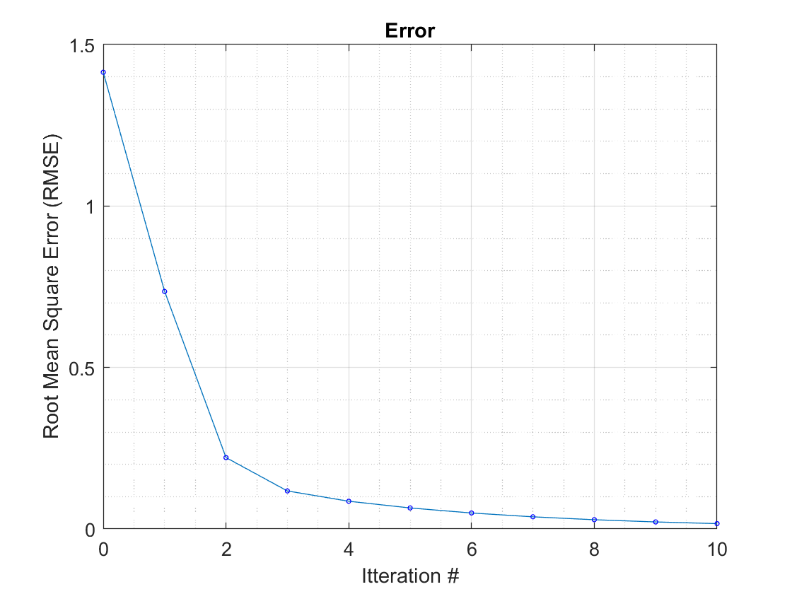
We can see it zig-zag it’s way towards the center. Getting closer with every step. If we plot it’s error we can see it converging.

Newtons Revenge

A few weeks ago I had a post covering Newtons Method (Link). It’s an iterative root finding algorithm, which means it finds when a function equals 0.

$x_{n+1}=x_n-\frac{f(x_n)}{f'(x_n)}$

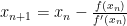
That doesn’t directly let us minimize a function, but lets think back to calculus 1. when the derivative of a function equals 0, the function is at a local minimum or maximum. This means that we can use newtons method to find where the derivative equals 0.

$x_{n+1}=x_n- \frac{f'(x_n)}{f''(x_n)}$

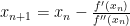
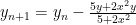
Using this on our above function means we would have the following update equations

$x_{n+1}=x_n - \frac{x+2xy^2}{1+2y^2}$

$y_{n+1}=y_n - \frac{5y+2x^2y}{5+2x^2}$

We can see that the gradient descent and the newtons method both converge to the same point, but they take different routs to get there. Why? Because the newtons method incorporated more information in the form of taking the second derivative. This gives it information about the curve and takes a more efficient route to the minima. It’s a second order method in comparison to the gradient descents which is a first order method.

Downsides of Newtons Method

If Newtons method outperforms gradient descent, why is this post on gradient descent? Because the second derivative that gives Newton’s method it’s advantage, is often extremely expensive to calculate. Numerical methods are all about being “good enough”. In my post on finite differences we rarely get the real derivative, we get an approximation that’s good enough. Gradient descent often gets us to a point that’s good enough faster than using Newton’s method because newtons method will need to stop to calculate it’s second derivative. Additionally, with newtons method, as with any equation with a variable in a denominator, you will always need to be careful with singularities

Downsides of Gradient Descent

Now, you shouldn’t think that gradient descent is a silver bullet that can always be used.

Let’s say we have a new cost function of the following form

$f(x,y) = (a-x)^2 + b(y-x^2)^2$

Through inspection we can easily see that as long as b is positive, this function will always be equal to or greater than zero. Also assuming b is positive, we can see that the only spot that this function will be zero is when

$(x,y) = (a,a^2)$

Let’s set a and b equal to 1 and 100 respectively and see how gradient descent would fare with an initial guess at (-.6,-.5)

Gradient descent starts off extremely quickly taking large steps but then becomes extremely slow. This is because the gradient approach is incredibly shallow. It doesn’t even come close to the real minima, (1,1), before progress turns into a crawl. Note: the name of this function is called the Rosenbrock function.

Think Global, Act Local

Let’s take a moment to talk more generally about optimization. In optimization, we want to find either a minimum or a maximum. Note: we can always re-frame the search for a maximum of a function f() as the search for the minimum of the function -f() and visa versa. Because of this I’ll now only talk about minimization.

In a bounded function, there will always be a some combination of inputs that minimize it. This is called the global minimum. There are also certain points that when you are nearby them, they seem like minimum, but aren’t. Let’s say we have the following function.

We can see that point A is clearly our global minimum, but if we were zoomed in at point B, it looks like it’s the global minimum. Gradient descent is like a ball rolling down a hill, so let’s image two balls, shown in green placed on the function and see where they roll to.

Because of their starting points, they both converge upon the local minimum instead of the global minimum. Gradient descent cant tell the difference between local minimum and a global one. How can you be sure you’re at the global minimum using gradient descent? You could drop a lot of balls, and hope that one of them reaches the global minimum, but how many balls would be enough? Additionally this gets extremely expensive, extremely quickly in higher dimensions. Optimization is a major problem in engineering and a lot of extremely clever people have come up with clever solutions for certain problems, but there is no one magic bullet that will work every time and definitely get you a global minimum. I’ve heard that this is a good book if you are interested in delving deeper on optimization.

Return to the Real World

I feel like I’ve gone too deep into the weeds of gradient descent without properly motivating why we would want to minimize a function. Outside of class, I’ve never run into a problem where there’s a single right answer that we’re solving for. Instead we’re trying to find a solution that satisfies some set of constraints.

Instead of trying to solve

$x + y = 1$

$x - y = 2$

where there’s one solution, we instead need to solve

$xy+y^2=1$

$xy > 0$

where there’s an infinite number of solutions, but y’s are expensive, so we want to minimize our y.

In my sub field, astrodynamics, we are often concerned with the amount of delta-V (Think fuel) it would take to get from one place (say earth) to another (say the moon). Unfortunately we want to minimize the delta-V while still getting to our destination in a reasonable time frame. It’s great if we can design a trajectory that gets us to our destination at a fraction of the delta-v, but it’s useless if the journey takes years instead of days if we have astronauts on board.

Want more Gerehses…

If you want to receive the weekly Gereshes blog post directly to your email every Monday morning, you can sign up for the newsletter here!

If you can’t wait for next weeks post and want some more Gereshes I suggest

The Math behind swinging a swing

Newton’s Method

My Undergraduate EDC