How to Pump a Swing Using Math - Dynamic Systems

Introduction

Growing up I really liked swings. I liked to pump the swing up as high as I could go. Young me would always try to go over the top pole for a full 360 degree swing. Unfortunately, I never went fast enough and the chain link arms, holding the seat to the pole, would collapse before I got over the top. It’s been a while since I’ve last been on a swing, or even thought about them, but they came up in a very strange place. My nonlinear controls class. The first assignment in my nonlinear controls class was to read through a paper called “How to Pump a Swing” by Stephen Wirkus, Richard Rand , and Andy Ruina.

Math Background

Note: None of the math in this section is new, I’m just going to paraphrase the article linked to above. If you have read through the paper already feel free to skip to the simulation section where I go over how to implement this model in Matlab.

Standing Pump

Lets model the swing as a pendulum with the rider being a mass at the end of the pendulum with mass m. The distance from the fulcrum point to the riders center of mass is L. Conservation of angular momentum for a point mass in a plane can be represented by the following equation:

$\frac{dH}{dt}=N$

Where H is angular momentum, and N is the net torque , both with respect to the fulcrum. The angle of the pendulum to the ground is phi, Φ, and the only force acting on the mass is gravity. By expanding out the angular moment of the body, mL^2 Φ, and the moment caused by gravity, -mg sin(Φ) we get the following equation.

$\frac{d}{dt}(L^2\dot{\phi})=-gl\sin\phi$

The rider begin every swing squatting and as they pass through Φ = 0 they immediately stand up. When stands to pump the swing, we can represent that as L getting a small amount shorter. This change in L happens in an extremely small change in time and therefore over an extremely small value of Φ. Integrating the conservation of angular momentum over this extremely small period of time gives us the following equation.

$L^2_{Stand}\dot{\phi}^+- L^2_{Squat}\dot{\phi}^- = -\int_{t_0}^{t_0+\Delta t} gL\sin\phi dt$

Where the superscript + and – denote standing and squatting respectively. As we make the increment of time smaller, the sine term in the integral goes to 0 and we get the following algebraic relation

$\dot{\phi}^+=\bigg(\frac{L_{Squat}}{L_{Stand}}\bigg)^2\dot{\phi}^-$

Sitting Pump

In order to simulate pumping in a sitting position we now need to make our model a little more complicated. Instead of a pendulum with a fixed mass but a changing length, we now have a pendulum with a barbel tied to the end of it. The angle that the barbel make with the rope is Θ, and each end of the barbells displacement from the center of mass is a. We can now rewrite conservation of angular momentum as

$\frac{d}{dt}\bigg[(L^2+a^2)\dot{\phi}+a^2\dot{\theta}\bigg] = -gL\sin\phi$

The rider has a Θ of 90 degrees when they are swinging forward and a Θ of 0 when swinging backwards. They change position when their angular velocity goes to 0. By integration over the last equation in a similar manner to what we did with the standing pump we get the following relationship to relate the amplitudes before and after changing position.

$\phi^+ - \phi^-=\frac{a^2\pi}{2(L^2+a^2)}$

Comparison of the Two Approaches

Through visual comparison of the two relationships, we can see that the standing pump increases the angular velocity of the rider by a multiple of the old velocity. The sitting pump increases the angular position by a fixed amount every time. This means that at small velocities the sitting pump is more efficient but is overtaken by the standing pump once the velocity is large enough.

Simulation

Now that we have looked into the analytical analysis of the problem, lets create some graphs using numerical integration. The graphs we will be generating are called phase plots. Unlike a normal time vs position plot, these will have the angular position as their X axis, and angular velocity as their Y axis. These type of plots are extremely useful when studying dynamic systems, as they allow us to see how the states trajectories evolve. If we plot several of these trajectories, all with different initial conditions, we get a phase portrait. I will be working in MatLab using ODE45 as my numerical integrator.

Naive Approach

If we look at the above math for the standing pump, we notice that the rider is standing whenever the sign of the riders angular velocity is the same as the sign of their angle.

$\begin{cases}Standing & \theta*\dot{\theta}\le0\\ Squatting& \theta*\dot{\theta}<0\end{cases}$

I placed this piece wise equation into the ODE function as an if-else statement and then ran it through ODE45. I got the following state space graph for initial conditions of

$\theta = -.1 , \dot{\theta}=0$

While this graph does show the proper outward spiral we would expect we also see that it’s continuous. The analysis done in the paper shows that it shouldn’t be continuous, but have discrete jumps at Φ= 0. What gives? To be honest, I’m still not sure. I talked with my professor and he thinks that it is ODE45 doing something weird behind the scenes.

Using Events with ODE45

Now that our naive approach has failed, lets move on to plan B, event functions. Event functions allow you to break out of the ODE function when a state achieves a certain value. Here we are going to use them to breakout of the function whenever Φ = 0. Then, using the analytical relationship discussed above , we will update the angular velocity. With the new corrected angular velocity we are going to start ODE45 again using the new angular velocity as the new initial conditions. This will allow us to have our jump continuities. Starting at the same initial conditions we get

Here we get the correct jump discontinuities. Additionally, we see the energy in the system increases proportionally to the amount of energy already in the system. This was not present in the naive approach. Lets now overlay the graphs of the two results.

Above we can see that whatever was affecting the naive approach made it so that the initial results are much smaller in final energy even though they had the same initial conditions, integration time, and system parameters. Just for completeness lets zoom in on the overlapping sections.

Would we have caught that ODE45 mistake from the naive approach if we had not analytically looked at the problem first? Probably not for a while. A little time with pencil and paper working through the problem can often save a lot of time while trying to debug simulations.

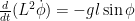
We can again use events for simulating sitting pumps and we would get the following graph (please note this was simulated with different initial conditions)

All code used in this post can be found here.

Reality

Now that we know that pumping a swing while standing is more effective at larger amplitudes one question should be present in your head. Is there anyone that takes advantage of it? This theory is nice but if no practices it, could there be some hurdle to a standing pump in reality. As it turns out it is practiced in the Estonian sport of Kiiking, a video of which is shown below.

I kinda want to go find a swing now!

How to Pump a Swing Using Math – Dynamic Systems