An Introduction to Finite Difference

What’s a Finite Difference and Why do we Want it

A common situation in real world problems is you have to take a derivative, but you don’t have the underlying function. You might be measuring some natural phenomenon and then only have discrete data points. Another time you wont be able to get a general derivative is where calculating the derivative would be prohibitively expensive. In those cases, we can turn to a finite difference.

Note: Hey, The last post on numerical methods, An Introduction to Newtons Method, was a surprise hit, being catapulted to the second most read post on this site. I’ll be producing more numerical methods posts in the future, but if you want to get ahead, I recommend this book.

Backwards from Calculus

The finite difference, is basically a numerical method for approximating a derivative, so let’s begin with how to take a derivative. The definition of a derivative for a function f(x) is the following

$\frac{df(x)}{dx} = \lim_{h\to0} \frac{f(x+h)-f(x)}{h}$

Now, instead of going to zero, lets make h an arbitrary value. To mark this as difference from a true derivative, lets use the symbol Δ instead of a d.

$\frac{\Delta f(x)}{\Delta x} = \frac{f(x+h)-f(x)}{h}$

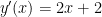
If we were to make h tend towards 0 we would return to our traditional definition of a derivative. But what is h? Let’s again go back to a simple description of what is a derivative of a function. It’s the slope of a function at a point. If we wanted to find the slope of a line, m, we would use the following formula

$m= \frac{f(x_2)-f(x_1)}{x_2-x_1}$

So, for a line, these two functions should be the same

$\frac{f(x+h)-f(x)}{h}=\frac{f(x_2)-f(x_1}{x_2-x_1}$

For a line we can see that h is just the difference between the two points we chose, but what about some random curve?

In the above figure we are taking the derivative of the green point and the red line is the actual derivative.

Now, if we pick two random points and use the slope formula we can see that this derivative, shown in yellow below, does not come close to being a good approximation to the real derivative.

Let’s try again, this time choosing two points really close to where we want to take our derivative. We want to get really close so I’ve zoomed in on the function.

Our curve looks more like a line when we zoomed in and our new numerical difference seems to be extremely close to the actual derivative. If our function is smooth and continuous, then when we zoom in on it enough it will usually look like a line. Now our slope formula begins to approach a good approximation of the derivative.

Note: taking the forward difference of a function f at a certain point t is commonly shown as the following

$\Delta f(t) \approx \frac{df(t)}{dt}$

How Good of a Job Does it Do?

Heuristically, we know that the smaller our h, the closer our appropriation is to the actual derivative. Does it approach it linearly, quadratically, asymptotically? Let’s explore it through a Taylor series expansion. Let’s expand our general function f(x).

$f(x+h) = f(x)+f'(x)h+\frac{f''(x)h^2}{2}+\sum_{i=3}^\infty \frac{f^i(x)h^i}{i!}$

In order to put it into the same form as our forward difference, we can subtract f(x) from both sides

$f(x+h)-f(x) = f'(x)h+\frac{f''(x)h^2}{2}+ \sum_{i=3}^\infty \frac{f^i(x)h^i}{i!}$

Now let’s divide both sides by h

$\Delta f(x) = \frac{f(x+h)-f(x)}{h}=f'(x) +\frac{f''(x)h}{2} +\sum_{i=3}^\infty \frac{f^i(x)h^{i-1}}{i!}$

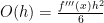
Now that we have our finite difference, lets define some error function O() and see how it varies with h.

$O(h) = -f'(x) + \Delta f(x) = -f'(x) + f'(x) + \frac{f''(x)h}{2} + \sum_{i=3}^\infty \frac{f^i(x)h^{i-1}}{i!}$

This simplifies to

$O(h)=\frac{f''(x)h}{2} + \sum_{i=3}^\infty \frac{f^i(x)h^{i-1}}{i!}$

Because we know h is small, anytime it’s raised to a high power it gets even smaller. This means that O(h) will be dominated by the first term and we can neglect those latter terms. This simplifies our error function down to

$O(h)=\frac{f''(x)h}{2}$

Which we can see varies linearly with h. This means that in order to halve our error, we need to half our step size. This is good but can we do better?

Note: This section of the post, analyzing a numerical method, is an extremely important part of numerical methods. Dover has a cheap book that focuses on analyzing numerical methods. It would make a good introduction to the topic if you found this section interesting.

Back to the Future

First let’s take a brief aside to what happens if h is negative? Our finite difference would then be

$\frac{y(x-h)-y(x)}{-h}$

Instead of taking the difference of the point we want, g, and a point some value h in front of our desired point, we’re now taking the difference of the point we want and a point some value h behind our desired point.

This is called the backwards difference and is represented as the following.

$\nabla f(t) \approx \frac{df(t)}{dt}$

Forward difference, backwards difference, and actual derivative, represented in blue, red, and green respectively.

I’ve drawn the both the forwards and backward difference above. You should verify that the absolute value of the error for the backwards difference is the same as the error for the forwards difference.

Stuck in the Middle With You

Now, let’s get back to the question of can we do better than a forwards difference? Let’s setup the following function

$y(x) = x^2+2x+1$

We can calculate it’s derivative exactly as

$y'(x)=2x +2$

If we want to find the derivative at x=2 we know that it would be 6. Let’s see how our forward and backward difference stack up with an h of .1

y'(2) = 6
Δy(2)=6.1
∇y(2)=5.9

So we can see that both are off, but if we averaged them together they would be the actual value in this case. What if we more generally averaged the forward and backwards distance together and then algebraically manipulated it to reduce terms.

$\frac{\Delta f(t) + \nabla f(t)}{2} = \frac{1}{2}\big( \frac{f(t+h)-f(t)}{h} + \frac{f(t-h)-f(t)}{-h}\big)=\frac{f(t+h)-f(t-h)}{2h}$

This is called the central difference and it can be denoted a bunch of ways, but for now let’s denote it with a δ.

$\delta f(t) = \frac{f(t+h)-f(t-h)}{2h}$

Error of the Central Difference

In order to calculate the error in the central difference, we’re going to again resort to a Taylor series expansion, but now lets have the stated terms go out to the third power.

$f(x+h) = f(x)+f'(x)h+\frac{f''(x)h^2}{2}+\frac{f'''(x)h^3}{6}+\sum_{i=4}^\infty \frac{f^i(x)h^i}{i!}$

Let’s do the same thing with the backwards difference term

$f(x-h) = f(x)-f'(x)h+\frac{f''(x)h^2}{2}-\frac{f'''(x)h^3}{6}+\sum_{i=4}^\infty \frac{(-1)^i f^i(x)h^i}{i!}$

Note that when -h is raised to an even power, the sign for that term is positive.

Subtracting the backwards difference from the forwards difference we get

$f(x+h)-f(x-h) = 2f'(x)h + \frac{2f'''(x)h^3}{6}+\sum_{i=4}^\infty \frac{(1-(-1)^i) f^i(x)h^i}{i!}$

dividing both sides by 2h will give us our central difference

$\delta f(x) =\frac{f(x+h)-f(x-h)}{2h}=f'(x)+ \frac{f'''(x)h^2}{6}+\sum_{i=4}^\infty \frac{(1-(-1)^i) f^i(x)h^{i-1}}{2(i!)}$

Let’s again define an error function O() as a function of h

$O(h) = -f'(x)+\delta f(x) = \frac{f'''(x)h^2}{6}+\sum_{i=4}^\infty \frac{(1-(-1)^i) f^i(x)h^{i-1}}{2(i!)}$

Once again we can neglect the higher order terms if h is small so we get the following

$O(h) = \frac{f'''(x)h^2}{6}$

Which we can see is quadratic with h. This means that if we cut our step size h in half, the new error is now a quarter of it’s old value. This is highly valuable because we now get a better approximation than a forward difference for an equivalently sized h.

Higher Order Difference

What if we want to take a second derivative of a function?

We want to find f”(x) which can be represented as the following

$f''(x)=\frac{d^2f(x)}{dx^2} = \frac{dg(x)}{x},$

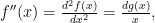
where

$g(x)= f'(x).$

Let’s use the central difference to approximate g'(x)

$f''(x) \approx \frac{g(x+h)-g(x-h)}{2h}= \frac{f'(x+h)-f'(x-h)}{2h}$

Now let’s replace our f'() with another central difference to get

$f''(x) \approx \frac{\frac{f(x+2h)-f(x)}{2h} - \frac{f(x)-f(x-2h)}{2h}}{2h} = \frac{f(x+2h)-2f(x)+f(x-2h)}{4h^2}$

We could repeat a similar procedure to obtain either higher order derivatives. Try now to derive a second order forward difference formula.

Asterisk Around Finite Difference

Let’s end this post with a word of caution regarding finite differences. Imagine you have the following function

$f(x)=\frac{1}{x^2}$

Whats the central difference using an h of 1 and at point x=0;

You should get δf(x)=0.

Now, using the quotient rule, get the actual derivative. You’ll see that at x=0 the actual derivative is undefined. Now try taking a forward or backwards difference and you’ll see that they are also undefined, like the actual derivative.

What gives? Isn’t the finite difference supposed to be more accurate than the forward or backwards difference? I don’t have the room in this post to go over when a finite difference can fail, but they are only approximations of a real derivative. They can fail and unless you are aware of their limitations can ruin your analysis. I’ll give you three quick rules of thumb for when you should be extra careful about using a finite difference.

You should always be careful using a finite difference near a singularity
You should also be careful using a central difference if your function is oscillatory.
Be aware of numerical error (I’m planning on going over numerical error as well as other sources of error in a future post, but for now here’s a link to Wikipedia)

Want more Gerehses…

If you want to receive the weekly Gereshes blog post directly to your email every Monday morning, you can sign up for the newsletter here!
If you can’t wait for next weeks post and want some more Gereshes I suggest

The Math behind swinging a swing

Newton’s Method

My Undergraduate EDC