Jacobi and his Constant - The 3-Body Problem

Recap

In the last two posts on what is the 3-body problem and the dynamics of the three body problem I’ve shown you the following GIF with a spacecrafts trajectory in the earth moon system. The trajectory is bouncing around what I’ve labeled a ‘forbidden region’. In this post we’ll go over the number behind that that forbidden region, the only constant of integration in the Circular Restricted 3-Body Problems, Jacobi’s Constant.

Note: this is an ongoing series on the CR3BP. If you want to get ahead on your own these are some good books on the material and astrodynamics in general (Book 1, Book 2, Book 3, Book 4).

One Integral to Rule Them All

Like most integrals of motion, we will begin with our equations of motion.

$\ddot{x} =2\dot{y}+x -\frac{(1-\mu)(x+\mu)}{d^3}- \frac{\mu(x-1+\mu)}{r^3} =2\dot{y} + \Omega*_x$

$\ddot{y} = -2\dot{x}+y-\frac{(1-\mu)y}{d^3}- \frac{\mu y}{r^3}=-2\dot{x} + \Omega*_y$

$\ddot{z} = -\frac{(1-\mu)z}{d^3}- \frac{\mu z}{r^3}= \Omega*_z$

where Ω*, the pseudo potential is defined as

$\Omega* = \frac{1-\mu}{d}+\frac{\mu}{r}+\frac{x^2+y^2}{2}$

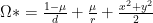
If we multiply each equation by it’s respective velocity and then add them together we get

$\dot{x}\ddot{x}+\dot{y}\ddot{y}+\dot{z}\ddot{z}= \Omega*_x\dot{x}+ \Omega*_y\dot{y}+ \Omega*_z\dot{z}$

expanding out the right hand side we get

$RHS = \frac{\delta \Omega*}{\delta x}\frac{dx}{d\tau} + \frac{\delta \Omega*}{\delta y}\frac{dy}{d\tau}+\frac{\delta \Omega*}{\delta z}\frac{dz}{d\tau}=\frac{d\Omega*}{d\tau}$

We can now integrate both sides by non-dimensional time τ to get the following relationship

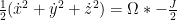
$\frac{1}{2}(\dot{x}^2+\dot{y}^2+\dot{z}^2) = \Omega*-\frac{J}{2}$

where J is Jacobi’s Constant. Why did I make it negative and divide it by two if it’s just some constant? So that we could rearrange the equation into

$J=2\Omega*-v^2$

where v is the magnitude of the velocity.

Looking into the Jacobi Constant

So what does the Jacobi constant tell us?

Ω is a function of position and μ, the mass ratio of the two major bodies.
v is only a function of velocity
J is a constant

This means our Jacobi constant relates our position to our velocity at any point. Let’s now create a contour map of the Jacobi values over the earth moon system. Note: we are going to do this by varying the position and keeping the velocity constant at 0. The color bar on the right identifies the Jacobi constant at a contour of that color.

Note: I’ve generally only plotted a range of Jacobi values to help show the contours some of these graphs are between 3 – 3.5 and others are between 3.0 – 4.0. The color bars are all correct.

μ’ve over

Earlier we said that v is funciton of velocity, and Ω is a function of both position and μ, the mass ratio of the two major bodies. Instead of plotting the Jacobi contours for a single system, let’s sweep through all the possible μ values. First let’s just remind ourselves what μ is defined as

$\mu = \frac{m_2}{m_1+m_2}$

Because our masses can only be positive, μ is bounded between 0 and 1

The first thing we should take away from that plot is that the Jacobi constant is mirrored across the X-Axis. Second is that the contours when μ is between 0-.5 is identical, but rotated 180 degrees around the barycenter to when μ is between 1-.5.

UnReal

Let’s all pretend we’re mathematicians for a moment and that we can get negative mass at the snap of a finger. Here’s what happens if we make mu negative

Neat. Useless, but neat.

Into the 3rd dimension

So far we have been exploring the Jacobi integral in two dimensions, X and Y, but we shouldn’t forget that it buried in r and d is a z component. If we mapped out the Jacobi constant for the earth moon system in the X-Z plane we get the following

Now lets sweep through the μ values again showing both projections at the same time.

You may have noticed that all the plots of the Jacobi contour are symmetric across the x axis. What if instead of plotting the X-Y view and the X-Z view on two separate plots, we combined them into one 2-D plot. The X axis will be the X-Axis and the positive portion of the Y-axis will have the X-Y contour, while the negative portion of the Y-axis will have the X-Z contour. This would make the Earth-Moon combined XYZ view the following

I’ve placed a thick red band across the center to demarcate the transition from the X-Y view to the X-Z view. What about if we now varied μ like we did in the previous Gifs?

Pretty neat right? Does it tell us anything useful? We can see that it’s continuous over the demarcation line, and that the change we see in the X-Z axis is coupled to the change in the X-Y axis. Even through I’ve been showing them in 2-D plots, the Jacobi contours are really 3-dimensional structures. Other than that, we don’t really get that much extra new information. This was one of several ways I tried to use the symmetry to visualize the change in both dimensions at once. I included it in this post so that you see how experimentation with different visualizations often goes. Finding cool new visualizations often requires you to try out tons of other visualizations that aren’t good/useful. When you’re working on a visualization always ask yourself does this provide additional insight?

Note: The code used to generate all visualizations in this post, aside from the first, can be found here.

Want more Gerehses …

If you want to receive the weekly Gereshes blog post directly to your email every Monday morning, you can sign up for the newsletter here! Don’t want another email? That’s ok, Gereshes also has a twitter account and subreddit!

If you can’t wait for next weeks post and want some more Gereshes I suggest

The Math behind swinging a swing

Newton’s Method

My Undergraduate EDC

Jacobi and his Constant – The 3-Body Problem