An Introduction to Stability

Note: This post is adapted from a lecture I gave to my undergrads. It’s focused on presenting the basics of stability for dynamical systems. The big question this lecture is intended to answer is what will
our system do if we perturb it a small amount? This is not a rigorous treatment and in some locations, I have traded being technically correct for being clear. If you want a rigorous treatment of the material I suggest a textbook.

Linear Systems

When our dynamics are linear, we can always write our state space in the following form

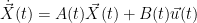
where is an n-by-1 state vector, A is a n-by-n state matrix , is a m-by-1 vector of controls, and B is a n-by-m input matrix.

Linear Stability

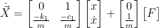
For the rest of this lecture, let’s pretend that our system has no controls. This leaves us with the reduced state space

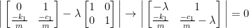
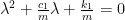
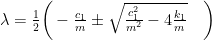
We can determine that our system’s stability by analyzing the eigenvalues, of the state matrix

where I is an n-by-n identity matrix.

Eigenvalue practice

Understanding eigenvalues

Now, each eigenvalue corresponds to a different behavior, and each eigenvector corresponds to a different mode

Positive Real Portion

An unstable system that goes to infinity in finite time (Technical term: Blow’s up)

Zero Real Portion some imaginary portion

This is called Marginally stable, never gonna stop, never gonna blow up, never gonna give you up

Negative Real Portion no imaginary portion

Stable (and simple)

Negative Real Portion some imaginary portion

Stable (and oscillatory)

Note: Eigenvalues with imaginary components always come in pairs of

Multiple Eigenvalues

If you have multiple eigenvalues, your system is dominated by the eigenvalue with the largest real portion. If the largest real portion is positive, your entire system is unstable. If your largest real portion of the eigenvalues is 0 your system is marginally stable. If your largest real portion of the eigenvalue is negative, the system is stable.

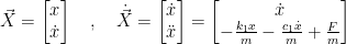
System of equations practice

Assume $m_1=m_2=1$

Assume that

Connecting Eigenvalues to a solution of ODE’s

We’ve seen that there’s a connection on which relates the eigenvalues of the state matrix and the stability of the system, but why is that? Let’s start this whole explanation off with a simple infinite series

Now let’s take it’s derivative with respect to x

The derivative of f is also f!

That’s such a nice property that we gave this function name e

Now, let’s return to differential equation land. The simplest linear differential equation is the following

Does this look familiar? Yes, it’s the same as our above equation (with some constants added), so we can say

Note: there’s this thing called a uniqueness proof which shows that for a linear ODE, this is the only solution. I wont go over it here, but just know we can rigorously prove that the exponential is the basic solution to a linear ODE.

Now that we have the solution for a single linear ODE, what about for system of linear ODEs? Instead of there just being a single exponential, the solution is the linear superposition of several of these base solutions

where , is the i’th eigenvalue, and , the i’th eigenvector.

Nonlinear Stability

Exploring stability, like most dynamics, is easy to do in linear systems. Extending it out to non-linear systems is less so. First we must define the concept of stationary points

Stationary Points

Stationary points are defined as states that satisfy the following condition

Stationary Points Practice

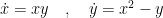
For the simple pendulum we have the following equation of motion, where all constants have been set to 1

This gvies us the following nonlinear state space

setting the derivative of the state vector to 0 we get the following two equations


Note there are an infinite number of stationary points for the humble pendulum, and we can mark each stationary point as .

Linearization

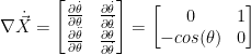
Let’s expand the derivative of our state vector about these stationary points using a Taylor series and then truncate the second order and higher terms

where indicates that you evaluate that term at stationary point . Now, at least for the region about that stationary point, we obtain the following relationship

We can now use the tools we developed for linear systems to determine the stability of stationary points.

Caveats About Linearization

Note: Because the linearization is only an approximation of the state matrix, you have to be aware of the following

• Linearization makes the assumption that we can approximate the derivative of the state vector by ignoring higher order terms. This is not always true! Explore the following example on your own
  
• This only covers a region close to the stationary point. How close? That depends on how important those higher-order terms we truncated are.
• While linearization can tell us if a stationary point is stable or unstable, if there is no real component (aka marginally stable), the results are inconclusive. The higher order terms can tip the system towards or away from stability.

Linearization Practice

Returning to our simple pendulum, let’s practice linearizing the system

Now, let’s get the eigenvalues when our pendulum is completely down and our pendulum is upright

which is marginally stable, so we would need a more advanced technique to determine the actual stability, but due to the nature of the symmetry we’ll find that it is truly marginally stable, and

which is clearly unstable as expected.

Want More Gereshes?

If you want to receive the weekly Gereshes blog post directly to your email every Monday morning, you can sign up for the newsletter here! Don’t want another email? That’s ok, Gereshes also has a twitter account and subreddit!