An Introduction to Direct Methods in Optimal Control

What is Optimal Control?

Lots of problems we encounter in the real world can be boiled down to “what is the best way to get from point A to Point B while minimizing a certain cost”. For a quadcopter, it’s how can I stay in my location while minimizing my battery usage. For a spacecraft, it’s how can I get from Earth to the Moon in the minimum amount of time to protect astronauts from radiation damage. In the GIF below, it’s how can I swing this pendulum on a cart upright using the minimum force squared. These problems are called optimal control problems and there are two main families of techniques for solving them, direct methods, and indirect methods. This post will go over the basics of setting up a direct method.

Cart Pole Swing up Gif

What are Direct Methods in Optimal Control?

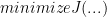
Direct methods in optimal control convert the optimal control problem into an optimization problem of a standard form and then using a nonlinear program to solve that optimization problem. The standard form that I will be using in this post is

$minimize J(...)$

$\boldmath{A} \vec{X} \le \vec{B}$

$\boldmath{A}_eq \vec{X} = \vec{B}_eq$

$C(\vec{X}) \le \vec{0}$

$C_{eq}(\vec{X}) = \vec{0}$

$lbd \le \vec{x} \le ubd$

A more general introductory tesxt to all optimal control can be found here

Discretizing the Trajectory

Let’s say we have some trajectory. The first task we have to do to put the trajectory in the standard form is to discretize it. I’m going to break the trajectory below into 3 distinct points.

At each of these points there’s a state X, a time t, and a control, U. We can stack them all together in several ways, but for this post, I’m going to choose the following.

$\begin{bmatrix} \vec{X}_1 \\ t_1 \\ \vec{X}_2 \\ t_2 \\ \vec{X}_3 \\ t_3 \\ \vec{U}_1 \\ \vec{U}_2 \\ \vec{U}_3 \end{bmatrix}$

for this example, let’s pretend that each state vector is made up of 3 states

$\vec{X} = \begin{bmatrix} x_1 \\ x_2 \\ x_3 \end{bmatrix}$

and each control vector is made up of 2 controls

$\vec{U}=\begin{bmatrix} u_1 \\ u_2 \end{bmatrix}$

There’s no set reason why I stacked the state and the time together and clumped all the controls at the bottom. We could have done it differently, we just need to keep track of where everything is. Additionally, to discretize problems in the real world we often need to discretize the trajectory into tens to even thousands of points depending on the difficulty of the problem.

Enforcing Boundry Constraints

For our trajectory, we don’t know what the path is going to be, but we do know where we want it to start, and where we want it to end. We can write these conditions for our 3 point discritization as

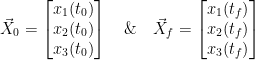
$\vec{X}_0 = \begin{bmatrix} x_1(t_0) \\ x_2(t_0) \\ x_3(t_0) \end{bmatrix} \quad \& \quad \vec{X}_f = \begin{bmatrix} x_1(t_f) \\ x_2(t_f) \\ x_3(t_f) \end{bmatrix}$

If we also have a set initial and final time, we can then write our boundary constraints as

$A_{eq}\begin{bmatrix} x_{1,1} \\ x_{1,2} \\ x_{1,3} \\ t_1 \\ x_{2,1} \\ x_{2,2} \\ x_{2,3} \\ t_2 \\ x_{3,1} \\ x_{3,2} \\ x_{3,3} \\ t_3 \\ \vec{U}_1 \\ \vec{U}_2 \\ \vec{U}_3 \end{bmatrix}=\begin{bmatrix} x_1(t_0) \\ x_2(t_0) \\ x_3(t_0) \\ t_0 \\ x_1(t_f) \\ x_2(t_f) \\ x_3(t_f) \\ t_f \end{bmatrix}$

where

$A_{eq} = \begin{bmatrix}I(4) & 0(4,4) & 0(4,4) & 0(4,6) \\ 0(4) & 0(4,4) & 0(4,4) & 0(4,6) \\ 0(4,4) & 0(4,4) & I(4) & 0(4,6) \end{bmatrix}$

and I(n) is the square identity matrix of size n, and 0(m,n) is a zero matrix of shape m rows and n columns.
Note: There’s no reason why we have to specify all these boundary conditions. For example with the pendulum swing up case shown in the gif in the top, we specified all the initial and final states, but we only care that at the end the pendulum is inverted. We could drop our final location requirement for the cart and this would also be a completely acceptable optimal control problem. It would, however, produce a different solution.

Enforcing The Forward Flow of Time

In this problem, we are enforcing an initial and final time, but let’s also enforce that time must flow forward. This constraint can be written generally as

$t_{n-1}<t_n <=> t_{n-1}-t_n<0$

or in the form of our nonlinear program

$A \begin{bmatrix} x_{1,1} \\ x_{1,2} \\ x_{1,3} \\ t_1 \\ x_{2,1} \\ x_{2,2} \\ x_{2,3} \\ t_2 \\ x_{3,1} \\ x_{3,2} \\ x_{3,3} \\ t_3 \\ \vec{U}_1 \\ \vec{U}_2 \\ \vec{U}_3 \end{bmatrix} \le \begin{bmatrix} 0 \\ 0 \\ 0 \end{bmatrix}$

where

$A = \begin{bmatrix} 0(1,3) & 1 & 0(1,3) & -1 & 0(1,10) \\ 0(1,7) & 1 & 0(1,3) & -1 & 0(1,6) \end{bmatrix}$

Note: we don’t always need to enforce forward time. Sometimes the best solutions are gotten by running the problem backward in time, but in most problems, it’s an unwritten constraint that we expect the final time to come after the initial time.
Note 2: In our problem, we specify both the initial and final times, but in problems where we allow the final time to vary, nonlinear programming solvers often want to run backward in time.

Enforcing Path Constraints

We can enforce simple path constraints on the states or the controls directly by imposing hard bounds on them.

$lbd \le \vec{x} \le ubd$

This is extremely useful because control in our optimal control problem is often bounded in real life. For example, spacecraft thrusters have hard limits on how much they can thrust.

Defects

Now we need to including the dynamics. Let’s jump back to differential equations and remember the following fact.

$x_{i+1}^I=x_i +\int_{t_i}^{t_{i+1}}\dot{\vec{x}}(t) dt$

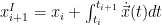
All this says, is that by integrating the derivative of the state vector over some time and combining it with the state vector at the start of that time period, we get the state vector at the next time period. But we already have a state at the next time period, so we call the difference between that, and what we get from integrating, the defect .

$\delta_i = x_{i+1}- x_{i+1}^I=x_{i+1}-x_i +\int_{t_i}^{t_{i+1}}\dot{\vec{x}}(t) dt$

By ensuring these defects are 0, we can ensure that all our different points are valid solutions to the dynamical system. We can do that using the nonlinear equality constraints

$C_{eq}(\vec{X}) = \vec{0}$

Bringing it all Together

In 2-body orbital dynamics, we can describe the relative motion of two close objects, where one is in a circular orbit using the Clohessy-Wiltshire equations, which are as follows

$\ddot{x} = 3n^2x+2n\dot{y}$

$\ddot{y} = -2n\dot{x}$

$n = \sqrt{\frac{\mu}{a^3}}$

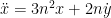
where mu is the gravitational parameter, and a is the radius of the target. This is extremely useful for final rendezvous with objects like the space station, which has almost no eccentricity. I’ve set up and then solved an optimal control problem of one satellite intercepting another satellite using the direct methods described in this post. The code for that can be found here (templateInit.m is the main script), and is mainly a wrapper around Matlab’s fmincon. Here’s a gif of the results.

Want more Gereshes?

If you want to receive new Gereshes blog post directly to your email when they come out, you can sign up for that here!

Don’t want another email? That’s ok, Gereshes also has a twitter account and subreddit!