

Inverted Pendulum Recap
In this post, we’re going to talk a little about how to balance an inverted pendulum on a cart. This is the second post in a 3 part series about balancing an inverted pendulum
- Part 1 – Balancing an inverted pendulum
- Part 2 – Swing-Up of an Inverted Pendulum on a Cart
- Part 3 – Kapitza’s Pendulum
Equations of Motion
Let’s start as we often do, by draw a diagram.

We’re going to acquire the equations of motion through the Lagrangian approach. This requires us to break up the problem and find the kinetic and potential energy for both the cart and the pole. First, let us start with the cart because it’s easiest. The cart can only move horizontally so its potential energy is 0

Its kinetic energy is also simple to write out

where M is the carts mass. Turning to the pole, it’s potential energy is
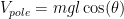
where m,g, and l are the mass at the end of the pole, the gravitational force, and the poles lengths. Unfortunately, the poles kinetic energy is a bit more complex as it interacts with the cart.
We can then combine these to form the Lagrangian

Using the following Euler-Lagrange equation,

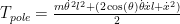
and then after an annoying amount of algebra, we arrive at the final set of equations
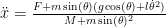

Where F is the force on the cart.
How are we Going to Control it?
In past posts on control, we’ve focused on looking at guiding our object to a destination from the entire phase space. In common terms, this means we could start the pendulum with any angular position and velocity and using the pendulums current state, compute a control that would make it stand upright. Unfortunately, now we have a much more complicated system and finding a global controller is much harder. Instead, let us make a simple assumption; we’re starting with the cart at rest, and the pendulum at rest hanging down. Now, we only need to find the control inputs that guide the pendulum to stand upright solely from the stated starting position, and not from any initial condition. By changing from a global solution to a single initial condition we have gone from designing a controller/policy to designing a trajectory.
The Lede

Trajectory design, while simple to say, actually covers a wide range of topics and techniques and I couldn’t figure out how to fit them, the methods, as well as how I used them here in this post, so instead I’m planning on having separate posts on things like collocation and non-linear programming. Once we have a foundation built up, I plan on returning to showing how to solve the swing-up problem. If you want a jump start on the topics I highly recommend this book on trajectory design.
Want More Gereshes?
If you want to receive new Gereshes blog post directly to your email when they come out, you can sign up for that here!
Don’t want another email? That’s ok, Gereshes also has a twitter account and subreddit!