Optimal Control of a Lunar Lander

Intro

Last year we had a 2 part series on how to land on the moon using a suicide burn. There, the condition was that we could only turn on the engine once, and it had to be fully throttled. But most landers can control their thrust, so in this post we’re going to go over how we could land the lunar lander using optimal control theory.

What is Optimal Control?

If you ever hear the word optimal, you should always be prepared to ask “With respect to what?”

Imagine we were car shopping and we needed to choose between a Tesla Model S and a Chevrolet Cruze. The Tesla is faster than the Cruze, but the Cruze costs a lot less. If we were purchasing a car only based on price, the Cruze would be the optimal choice. Visa-Versa, if our purchase was only based on speed the Tesla would be the optimal choice. But in the real world, we rarely do something only based on one parameter. We want both high speed and low cost so we need some way to measure them together. We could define a cost function, J, that takes both into account. An example cost function could be

$J = \alpha P_{rice} + \frac{\beta}{S_{peed}^2}$

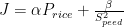
where α and β are constants showing how important that feature is to us. We could plug the Tesla’s and Cruze’s stats into this equation and the one with the lower cost function would be the optimal one for us. We could add in more features to our cost function like lifetime cost, resale value, etc… and that would allow us to pick the optimal car out of all the possible cars for us. The problem is that these cost functions are not unique. In this car example, they are defined by the needs of the person driving the car. What’s optimal to me, a poor grad student, would be different than what’s optimal for a millionaire.

So what is optimal control? It’s a branch of control theory that focuses on finding a control law to optimize an arbitrary cost function. It grew out of the calculus of variation and is too large a topic to go over in a single class, much less a single post, but for now the main take away for you should be:

Optimal Control is about controllers that optimize an arbitrary cost function J

Note: The rest of this post is going to be me working though the landing problem. I’ll be stating what I’m doing, but I wont be going over the why this ensures optimal. That will be for a future post on Pontryagin’s maximization principle. If you’re interested in a good introductory book on Optimal control I suggest this one . It’s what I used to teach myself the basics of optimal control for a research project I’m working on.

Onto The problem

So let’s create a free-body diagram of our lander

We have two forces acting on it, a constant gravitational force and the variable thrust force. We can control the angle, θ, of the thrust directly. This leads us to our equations of motion

$\boldsymbol{\dot{r}}=\boldsymbol{v}$

$\boldsymbol{\dot{v}}=\frac{c_1 u_1}{m}\boldsymbol{\hat{i}_\theta}+\boldsymbol{g}$

$\dot{m}=\frac{-c_1}{c_2}u_1$

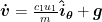
where g is the moons gravity, m is the spacecrafts mass, c1 is the max engine thrust in newtons, and c2 is the engines efficiency.

A Cost function and Hamiltonian

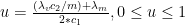
Let’s first define a cost function. we want our lander to use the smallest amount of thrust possible so we can define our cost function as

$J = \int_0^{t_f}u^2 dt$

I set it up as the thrust squared, because that makes our cost function quadratic. The smallest possible number that our cost function can take on is 0 if we don’t thrust at all and can only grow. This makes the convergence a little nicer later on. Now, because i’m going to use Pontryagin’s maximization principle I’ll define the following Hamiltonian

$H = \boldsymbol{\lambda}_r\cdot\boldsymbol{v} + \boldsymbol{\lambda}_v\cdot\boldsymbol{\dot{v}}-\lambda_m\frac{c1}{c2}u + u^2$

Control law

Now that we have our Hamiltonian, we can find our control laws by the following relationships

$\frac{\delta h}{\delta \theta} = 0$

$\frac{\delta H}{\delta u}=0$

Which gives us

$\boldsymbol{\hat{i}}_\theta =-\frac{\boldsymbol{\lambda_v}}{\lambda_v}$

and

$u = \frac{(\lambda_v c_2 / m)+\lambda_m}{2*c_1} , 0 \leq u \leq 1$

Co-State Equations

We’ve derived the equations of motion and the control laws, but what about those λ that popped up in our control laws? They can be found through the following relationship

$\dot{\lambda}_q = \frac{-\delta H}{\delta q}$

which give us the following co-state equations

$\boldsymbol{\dot{\lambda}_r}=0$

$\boldsymbol{\dot{\lambda}_v}=-\boldsymbol{\lambda}_r$

$\dot{\lambda}_m=\frac{c_1}{m^2}\boldsymbol{\lambda}_v\cdot \boldsymbol{\hat{i}}_\theta u$

Note: The first two sets of co-state equations can be solved directly.

A Boundary Value Problem

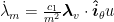
This leads us to the following set of equations

$\boldsymbol{\dot{r}}=\boldsymbol{v}$

$\boldsymbol{\dot{v}}=\frac{c_1 u_1}{m}\boldsymbol{\hat{i}_\theta}+\boldsymbol{g}$

$\dot{m}=\frac{-c_1}{c_2}u_1$

$\dot{\lambda}_m=\frac{c_1 u}{m^2}[(\lambda_{vx0}-\lambda_{x0}t)\sin\theta+(\lambda_{vx0}-\lambda_{x0}t)\cos\theta]$

We also need to satisfy the boundary conditions of r0,v0,m0 at t=0 and r(t)=(0,0),v(t)=(0,0), and λm(t)=0 at t=final time. There are many ways to solve this two point boundary value problem, but the one I’ve chosen is to use a shooting method, which I wrote about here.

And once again the spacecraft actually landing

I’ve plotted the thrust and direction using the blue arrows. You may notice that it doesn’t point up. If it doesn’t point up, how does it land? It does point up, it’s just not noticeable. If you look at the Y-Axis you’ll notice that it span’s thousands of meters while the X-Axis is only 8 meters. This was the only way to show the curvature of the trajectory, but it squishes down the upward thrust so it’s imperceptible. (I played around with a few other visualizations, but I didn’t like any)

Why this topic?

The math in this post was taken from a wonderful paper called “Real time Optmal Control via Deep Neural Networks: Study on landing problems” by Sanchez and Izzo. In it, they attempt to replicate the optimal control method we’ve gone over above with a neural network. They actually do a whole lot more than just this one landing scenario, I highly recommend reading that paper. I recreated that paper as a part of an active research project I’ve been working on. I want to experiment with using this blog as a more informal companion to my research so as I publish new work there may be new companion pieces here. If you like the idea or have suggestions, feel free to leave them in the comments below or email me at ari@gereshes.com!

Want More Gereshes

If you want to receive the weekly Gereshes blog post directly to your email every Monday morning, you can sign up for the newsletter here! Don’t want another email? That’s ok, Gereshes also has a twitter account and subreddit!

5 Comments

Karthi Ramachandran

2019-10-22

If u could help me understand the doubts
1) after u frame the Hamiltonian , why you differentiate the Hamiltonian w.r.t theta and u . Normally I read we differentiate with “u”.
2) what is lambdaVx0 and lambdaVy0 and how “t” came in the equation of lambdaMdot?
3) Are you using switching ?

please clarify in a mail if the questions are valid .
- admin
  
  2019-10-22
  
  1) In this problem, we have two control variables (u – our thrust, and theta – our angle) so we need to differentiate the hamiltonian with respect to both. In most texts, they just generalize all the controls to just be u. In this post I explicitly wrote out what they generally implicitly write.
  
  2a) lambdaVx0 and lambdaVy0 are lambdaVx and lambdaVy at the initial time.
  2b) Because they are linear equations they can be solved for explicitly in terms of time and we can plug those solutions into the equation for lambdaMdot to simplify our final equations
  
  3) No, not in this case
- Karthi Ramachandran
  
  2019-10-22
  
  i got answers for all three(hope you are not using switching) . could you share the how you choose the final time alone?
  - admin
    
    2019-10-22
    
    There are two main ways to find a final time. You can either be given a final time or you can implement a variable time shooting method (what I used in this paper). Both are rather trivial for the scenario in this post.
    - Karthi Ramachandran
      
      2019-10-22
      
      thank you

Comments are closed.