Introduction to State Space

Once you derive the equations of motion for a system, the next step in simulating it numerically is to compute the state-space representation, the backbone of modern contorl theroy. This is useful because by placing the equations of motion in a common format we can apply a whole host of techniques to study the system. Computing the state space is made up of 3 main steps

Determine the States
Determine the State Transitions
Determine the Measurement

Determining the States

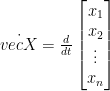
When we say determine the states, we want to find the minimum number of variables that we can use to represent the system for all time. Put another way, if we have a full set of state variables at one time, we could represent it at any other time. Take, for example, a ball in a gravity field. If we know it’s position and velocity at any point in time we could use the equations of motion to find its positions and velocity at any other time. If we only knew one piece of information, position or velocity, we could not determine the other. Let’s write an n state system together in a vector form as the following

$\vec{X}=\begin{bmatrix} x_1\\ x_2\\ \vdots \\ x_n \end{bmatrix}$

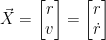
This is called our state vector. For a 1-D ball in a gravity field, our states would be a position r, and a velocity v. The state vector would be

$\vec{X} = \begin{bmatrix} r \\ v \end{bmatrix} = \begin{bmatrix} r \\ \dot{r} \end{bmatrix}$

Determine the State Transitions

In our definition of states, we said that given the full set of state information at one point in time, we want to figure out its state at another point in time. In order to do this, we need to find out how our state vector changes with time. This means taking the derivative of the state vector

$\dot{vec{X}} = \frac{d}{dt}\begin{bmatrix} x_1\\ x_2\\ \vdots \\ x_n \end{bmatrix}$

In the case of our 1-D ball, the derivative of our state vector would be

$\vec{X} = \begin{bmatrix} \dot{r} \\ \ddot{v} \end{bmatrix} = \begin{bmatrix} \dot{r} \\ \ddot{r} \end{bmatrix}$

We can then plug in our equations of motion

$\ddot{r} = L(r,\dot{r})$

In a slightly more general form, the derivative of our state vector can be written as the following

$\dot{\vec{x}} = f(t,\vec{X},u)$

Which means the derivative vector is some function of the time, the current state, and some external input, u.

Determine the Measurement Vector

This third component of a complete state-space representation is a bit rarer than the first two. It’s the measurement vector and comes up mostly in the field of estimation. Once again, it’s a vector and it relates your current, time, state, and some external input to what you would measure.

$\vec{y}=h(t,\vec{X},u)$

I don’t generally use the measurement vector, so, for now, let’s pretend it just doesn’t exist. For the rest of this whenever I say state-space representation I’m only going to discuss two parts

The state Vector, $\vec{X}$
The time derivative of the state Vector , $\dot{\vec{X}}$

Example Time: The Nonlinear Pendulum

Now that we have an idea what the state-space representation is, let’s practice on an example problem we’ve encountered on this blog before, the non-linear pendulum.

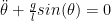
Here the equation of motion is as follows

$\ddot{\theta}+ \frac{g}{l} sin(\theta)=0$

The state vector for this problem are

$\vec{X}=\begin{bmatrix}\theta\\ \dot{\theta}\end{bmatrix}$

Taking it’s time derivative, and substituting in the equation of motion we get

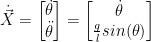
$\dot{\vec{X}}=\begin{bmatrix}\dot{\theta}\\ \ddot{\theta}\end{bmatrix}=\begin{bmatrix}\dot{\theta}\\ \frac{g}{l} sin(\theta)\end{bmatrix}$

We now have our pendulum in a state-space representation. A good sanity check is to add all the orders of the governing equation together and seeing if it matches the number of states. In this case, we have 1 2nd-order equation of motion and 2 states so we’re good.

Example Time: CartPole

Let’s now expand to a system which requires multiple coupled equations to describe it. I derive the equations of motion for the cart pole system here, so here they are re-produced without derivation

$\ddot{\theta} = (c_1+c_2)\theta-u$

$\ddot{x}=u-c_2\theta$

Now, we have constants in our equations of motion, c1 and c2, as well as some external input, u. Here the statespace representation is

$\vec{X} = \begin{bmatrix} \theta \\ x \\ \dot{\theta} \\ \dot{x} \end{bmatrix}$

$\dot{\vec{\theta}} = \begin{bmatrix} \dot{\theta} \\ \dot{x} \\ \ddot{\theta} \\ \ddot{x} \end{bmatrix}= \begin{bmatrix} \dot{\theta} \\ \dot{x} \\ (c_1+c_2)\theta-u \\ u-c_2\theta \end{bmatrix}$

Let’s now do our quick sanity check. We have 2 2-nd order differential equations so we should have four states, and we do so it passes our check.

Problem Set

I’ve uploaded a small problem set if you want to practice placing systems into state-space form

Problem 1

$\ddot{x}-(1-x^2)\dot{x} + x = 0$

Problem 2

$\ddot{x} = x- x^3$

Problem 3

$\ddot{x} = \frac{-x}{r^3},\quad \ddot{y} = \frac{-y}{r^3},\quad \ddot{z} = \frac{-z}{r^3}$

where,

$r=\sqrt{x^2 + y^2 + z^2}$

Problem 4

$\ddot{\theta}=(c_1+c_2)\theta - u,\quad \ddot{x}=u-c_2\theta$

I’ve created a short video working through them below

Want More Gereshes?

If you want to receive new Gereshes blog post directly to your email when they come out, you can sign up for that here!

Don’t want another email? That’s ok, Gereshes also has a twitter account and subreddit!