An Introduction to Shooting Methods

Intro/Motivation

One of the most common tasks in dynamics and controls is how do we get an object from point A to point B. Sometimes, like in the brachistochrone problem, we get lucky and there is a nice analytical solution. Unfortunately, in most situations, there is no closed form answer, and we need to turn to a numerical method. In our post on asteroid wars we turned to newtons method for a solution. Today we are going to generalize that method to deal with much more complicated problems.

Newton’s Method

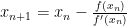
In an earlier post we talked about newton’s method. It’s an iterative way to find the roots of an equations. In Layman’s terms, what would make that equation equal 0. The update equation for Newton’s method is

$x_{n+1} = x_n - \frac{f(x_n)}{f'(x_n)}$

But how can we generalize it for dealing with multiple dimensions? What about instead of a single variable, x, we wanted to use it for a vector of variables, X? Well, let’s plug X in for x and see what happens

$\boldsymbol{X}_{n+1} = \boldsymbol{X}_n - \frac{f(\boldsymbol{X_n})}{f'(\boldsymbol{X}_n)}$

First thing we should notice is that we’re now dealing with vectors, so we cant just divide by a vector, instead we replace that division by a left multiplied inverse.

$\boldsymbol{X}_{n+1} = \boldsymbol{X}_n - f'(\boldsymbol{X})^{-1}f(\boldsymbol{X})$

Next, what does the single derivative f'() mean with vectors? Let’s replace that with a matrix of partial derivatives of the function with respect to the variables we can control. Let’s call that DF for now

$\boldsymbol{X}_{n+1} = \boldsymbol{X}_n - DF(\boldsymbol{X}_n )^{-1}f(\boldsymbol{X}_n)$

DF is defined as

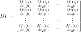
$DF = \begin{bmatrix} \frac{\delta f_1(t_f)}{\delta x_1(0)} & \frac{\delta f_1(t_f)}{\delta x_2(0)}& \cdots & \frac{\delta f_1(t_f)}{\delta x_n(0)} \\ \frac{\delta f_2(t_f)}{\delta x_1(0)} & \frac{\delta f_2(t_f)}{\delta x_2(0)}& \cdots & \frac{\delta f_2(t_f)}{\delta x_n(0)} \\ \vdots & \vdots &\ddots &\vdots \\ \frac{\delta f_m(t_f)}{\delta x_1(0)} & \frac{\delta f_m(t_f)}{\delta x_2(0)}& \cdots & \frac{\delta f_m(t_f)}{\delta x_n(0)}\end{bmatrix}$

When DF is square, it’s known as the Jacobin. This is a nice informal text on vector calculus, that covers topics like partial derivatives, Jacobians, etc… in more detail. I learned vector calc from this, but it’s a traditional expensive textbook.

Ok, So Now What?

We’ve generalized Newtons Method, but how do we now use that to solve a trajectory problem? Lets say we are at some state X_0 where we have a position and velocity, and we want to get to a different position X_d (for now let’s not care about our velocity at the final point)

Now, if we do nothing and let the system evolve for some time, we get a trajectory to our point X_f

These final states are a function of the initial states X_f(X_0), and we want to drive the difference between X_f and X_d to zero. We can rewrite that as the following function

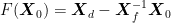
$F(\boldsymbol{X}_0)=\boldsymbol{X}_d-\boldsymbol{X}_f^{-1}\boldsymbol{X}_0$

which we can use the generalized newtons method to from earlier to drive it towards zero.

Time for an Example

So let’s use the shooting method on a simple example problem. Here’s a quick targeting problem. We have a cannon with a fixed location and we want to hit another fixed location. We can only adjust the initial velocity of the projectile.

First let’s define the F matrix

$F = \begin{bmatrix}x_d - x(t_f) \\ y_d - y(t_f)\end{bmatrix}$

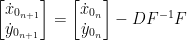
Where d subscripts are our desired targets and the f(t_f) is the function at the final time. If we then take the derivative of the F matrix with respect to our initial conditions

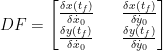
$DF = \begin{bmatrix} \frac{\delta x(t_f)}{\delta\dot{x}_0} && \frac{\delta x(t_f)}{\delta\dot{y}_0} \\ \frac{\delta y(t_f)}{\delta\dot{x}_0} && \frac{\delta y(t_f)}{\delta\dot{y}_0} \end{bmatrix}$

Note: I got the the terms in the DF matrix from a finite difference method. We can then use our generalized newtons method to drive our F matrix to 0.

$\begin{bmatrix} \dot{x}_{0_{n+1}} \\ \dot{y}_{0_{n+1}}\end{bmatrix}=\begin{bmatrix} \dot{x}_{0_{n}} \\ \dot{y}_{0_{n}}\end{bmatrix}-DF^{-1}F$

We can see that even though our initial guess is way off, the shooting method converges within 7 iterations to being within 10E-14 of the target. We can use a shooting method to get within machine precision of our target. Also Note how the error decreases quadratic. I went over quadratic convergence for Newton’s method here, and a similar argument can be done for the shooting method, because it is a multidimensional version of Newton’s method.

All the Colors of the Rainbow

There’s not just a unitary shooting method. In the problem above, we had fixed the integration time, but we could have make that an additional variable. Then it would be a variable-time shooting method. We could have broken up the trajectory into separate arcs to improve convergence. Then it would be a multiple shooting method. We could have changed the method a dozen different ways to tailor it to our problem. Shooting methods are extremely powerful tools for solving 2 point boundary value problems, but we should be aware that there’s more to the method than what was covered in this post.

Want More Gereshes

If you want to receive the weekly Gereshes blog post directly to your email every Monday morning, you can sign up for the newsletter here! Don’t want another email? That’s ok, Gereshes also has a twitter account and subreddit!