Double Spring Mass Systems & Matlab's ODE 45

Lissajous curves

From orbits around Lagrange Points, to double pendulums, we often run into a family of loopy, beautiful, curves. These are called Lissajous curves, and describe complex harmonic motion. In layman terms, Lissajous curves appear when an object’s motion’s have two independent frequencies. Today, we’ll explore another system that produces Lissajous curves, a double spring-mass system, analyze it, and then simulate it using ODE45.

FBD, Equations of Motion & State-Space Representation

We start every problem with a Free Body Diagram

The springs follow Hooks law, which says

$F_s = -K_s d$

where F_s is the force from the spring, K_s is the spring constant, and d is how far away from normal the spring has been stretched.

We can use hooks law to determine the forces acting on the two blocks (don’t forget the force of the second block acting on the first)

$F_1=(-K_1 d_1)+K_2(d_2-d_1)$

$F_2=-K_2(d_2-d_1) = K_2d_1 - K_2 d_2$

Then, appealing to newton’s second law, we can turn these into two second order equations of motion

$\ddot{d}_1=((-K_1 d_1)+K_2(d_2-d_1))/m_1$

$\ddot{d}_2= (K_2d_1 - K_2 d_2)/m_2$

We have 2 coupled, 2nd order equations. We can always convert m number of nth order differential equations to (m*n) first order differential equations, so let’s do that now. We’ll need a change of variables to differentiate the 2 2nd order equations, from the 4 1st order equations. Let’s use x_i, where i is a number from 1 to 4, and let’s denote the vector of them as X.

First let’s define x_1 and x_2 as the following

$x_1 = d_1$

$x_2 = d_2$

Next let’s define x_3 and x_4 as the derivatives of x_1 and x_2 respectively

$x_3 = \dot{x}_1$

$x_4 = \dot{x}_2$

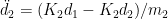
Now that we’ve done that, let’s figure out what the derivatives of x_3 and x_4 are

$\dot{x}_3=\ddot{x}_1 = \ddot{d}_1=[(-K_1 d_1)+K_2(d_2-d_1)]/m_1$

$\dot{x}_4=\ddot{x}_2 = \ddot{d}_2= (K_2d_1 - K_2 d_2)/m_2$

Let’s now sub in our x_i’s for any d’s

$\dot{x}_3=[(-K_1 x_1)+K_2(x_2-x_1)]/m_1$

$\dot{x}_4= (K_2 x_1 - K_2xd_2)/m_2$

Our system is linear, so let’s write it out in the following state space representation

$\dot{\boldsymbol{x}} = A \boldsymbol{x}$

$\begin{bmatrix} \dot{x}_1\\ \dot{x}_2 \\ \dot{x}_3 \\ \dot{x}_4 \end{bmatrix} = \begin{bmatrix} 0 & 0 & 1 & 0 \\ 0 & 0 & 0 & 1\\ \frac{-k_2-k_1}{m_1} & \frac{k_2}{m_1 } & 0 & 0 \\ \frac{k_2}{m2} & \frac{-k_2}{m_2} & 0 &0 \end{bmatrix}\begin{bmatrix} x_1 \\ x_2 \\ x_3 \\ x_4 \end{bmatrix}$

So why did we do all of that? Two reasons, linear analysis, and Numerical Methods

Linear Analysis

Because this is a linear system, we can find out a whole lot about it, just by looking at the A matrix

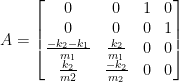
$A = \begin{bmatrix} 0 & 0 & 1 & 0 \\ 0 & 0 & 0 & 1\\ \frac{-k_2-k_1}{m_1} & \frac{k_2}{m_1 } & 0 & 0 \\ \frac{k_2}{m2} & \frac{-k_2}{m_2} & 0 &0 \end{bmatrix}$

If we took it’s eigenvalues, (and all the masses and spring constants were positive) we would find that we had four purely imaginary eigenvalues. This would tell use that once disturbed , the system will oscillate forever. The eigenvectors, would tell us about the different oscillation modes we could have. Because it’s linear and time invariant, we could determine the state transition matrix through a frequency domain analysis. I want to do a whole series on the basics of linear dynamics, so I wont go into detail here, but we could discover a whole lot from just that A matrix. Note: a cheap introduction to dynamic systems can be found here. A longer and more expensive, but very comprehensive book on linear systems can be found here.

Numerical Methods

Now that we’ve looked at what we can do if we have a linear system, what about if we don’t have a linear system? We can still put it into a state-space representation where it’s made up of (m*n) 1st order equations. That ability to reshape any set of differential equations into a common format makes it an ideal input for numerical methods. I’ve been asked a lot to go over the basics of how to input things for Matlab’s ODE45 so we’ll do that now.

Let’s first turn the state space equations of motion into a Matlab function. It take in time (t), the current states (X), and the extra arguments where we pass along the block’s masses and spring constants. Note that we return the states derivatives in a column vector.

function [xDot] = doubleSpringMass(t,X,args)
%State space fucntion of Double Spring Mass System
%Made for insert link to gereshes here
%Ari Rubinsztejn
%2018.12.22
x1=X(1);
x2=X(2);
k1=args(1);
m1=args(2);
k2=args(3);
m2=args(4);
F1=(-k1*x1)+(k2*(x2-x1));
F2=(-k2*x2)+(k2*x1);
x1DD=F1/m1;
x2DD=F2/m2;
xDot=[X(3),X(4),x1DD,x2DD]';
end

Now that we have our function, let’s write our wrapper script. Our initial conditions, ic, are in a vectors, as are our arguments, args. The time that we want to run our simulation for is in the vector ts where we specify the start and end times. We then plug it into ode45().

ic = [-1,3,0,0];
args=[4,1,4,1];
ts=[0,33];
sol=ode45(@(t,X) doubleSpringMass(t,X,args),ts,ic);

Note: I’m currently getting ode45’s output as a structure because it makes creating GIFS a bit easier. I’ve posted the rest of the code here on github that includes the section that generates the GIFs and images

Want more Gereshes

If you want to receive the weekly Gereshes blog post directly to your email every Monday morning, you can sign up for the newsletter here! Don’t want another email? That’s ok, Gereshes also has a twitter account and subreddit!

Double Spring Mass Systems & Matlab’s ODE 45