Stability of the Lagrange Points

Recap of Lagrange Points

In the circular restricted three body problem, there are a set of 5 points that if we place our spacecraft there, it’ll never move relative to the two bodies. These are called the Lagrange points and are the only equilibrium points for the system. Whenever we find an equilibrium point in a dynamic system the first question should always be “is it stable?”

Note: this is an ongoing series on the CR3BP. If you want to get ahead on your own these are some good books on the material and astrodynamics in general (Book 1, Book 2, Book 3, Book 4).

Linearized Equations of Motion

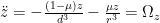
In order to investigate the stability of the Lagrange points, let’s write out the equations of motion.
$\ddot{x} = 2\dot{y}+x-\frac{(1-\mu)(x+\mu)}{d^3}- \frac{\mu(x-1+\mu)}{r^3} = 2\dot{y} + \Omega_x$
$\ddot{y}= -2\dot{x}+y -\frac{(1-\mu)y}{d^3}- \frac{\mu y}{r^3}=-2\dot{x}+\Omega_y$
$\ddot{z} = -\frac{(1-\mu)z}{d^3}- \frac{\mu z}{r^3}=\Omega_z$
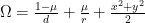
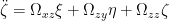
where Ω is defined as
$\Omega = \frac{1-\mu}{d}+\frac{\mu}{r}+\frac{x^2+y^2}{2}$
and Ω_n is just the derivative of Ω with respect to n.
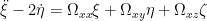
Let’s also define a perturbation off of any Lagrange point as the following
$x = x_{L_i} + \xi$
$y = y_{L_i} + \eta$
$z = z_{L_i} + \zeta$
Plugging these relations into our equations of motion and taking a first order Taylor series expansion to linearize our equations of motion we get
$\ddot{\xi}-2\dot{\eta}= \Omega_{xx}\xi+\Omega_{xy}\eta+\Omega_{xz}\zeta$
$\ddot{\eta}+2\dot{\xi} = \Omega_{xy}\xi+\Omega_{yy}\eta+\Omega_{yz}\zeta$
$\ddot{\zeta} = \Omega_{xz}\xi+\Omega_{zy}\eta+\Omega_{zz}\zeta$
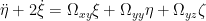
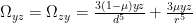
Where the double derivatives are as follows
$\Omega_{xx}= 1-\frac{1-\mu}{d^3}-\frac{\mu}{r^3}+\frac{3(1-\mu)(x+\mu)^2}{d^5}+\frac{3\mu(x-1+\mu)^2}{r^5}$
$\Omega_{yy}= 1-\frac{1-\mu}{d^3}-\frac{\mu}{r^3}+\frac{3(1-\mu)y^2}{d^5}+\frac{3\mu y^2}{r^5}$
$\Omega_{zz}= -\frac{1-\mu}{d^3}-\frac{\mu}{r^3}+\frac{3(1-\mu)z^2}{d^5}+\frac{3\mu z^2}{r^5}$
$\Omega_{xy}= \Omega_{yx}= \frac{3(1-\mu)(x+\mu)y}{d^5}+\frac{3\mu(x-1+\mu)y}{r^5}$
$\Omega_{xz}= \Omega_{zx}= \frac{3(1-\mu)(x+\mu)z}{d^5}+\frac{3\mu(x-1+\mu)z}{r^5}$
$\Omega_{yz}= \Omega_{zy}= \frac{3(1-\mu)yz}{d^5}+\frac{3\mu yz}{r^5}$
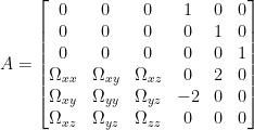
This means we can represent all of this in a nice, compact, matrix format
$\dot{\vec{x}}=\boldsymbol{A}\vec{x}$
$A = \begin{bmatrix} 0&0&0&1&0&0\\ 0&0&0&0&1&0\\ 0&0&0&0&0&1\\ \Omega_{xx} & \Omega_{xy} & \Omega_{xz} &0&2&0\\\Omega_{xy} & \Omega_{yy} & \Omega_{yz} &-2&0&0\\\Omega_{xz} & \Omega_{yz} & \Omega_{zz} &0&0&0\\ \end{bmatrix}$

Linear Systems are Nice

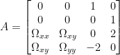
Now that we have a linear system, we can always determine the stability of said system by finding it’s eigenvalues. It’s also nice that because the z component is uncoupled from the x and y components, we can actually remove it and solve it on it’s own so we only need to find the eigenvalues of the following A matrix
$A = \begin{bmatrix} 0&0&1&0\\ 0&0&0&1\\ \Omega_{xx} & \Omega_{xy} &0&2\\\Omega_{xy} & \Omega_{yy} &-2&0\end{bmatrix}$
We know the eigenvalues of this matrix will be the roots to the following equation
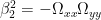
$\lambda^4 + (4-\Omega_{xx}-\Omega_{yy}) \lambda^2+ (\Omega_{xx}\Omega_{yy}-\Omega_{xy}\Omega_{yx})=0$
It’s form also allows us to reduce the equation from a quartic equation to a quadratic equation and introduce some coefficients
$\Lambda ^2 + 2\beta_1 \Lambda - \beta _2^2=0$
where
$\beta_1 = 2-\frac{\Omega_{xx}+\Omega_{yy}}{2}$
$\beta_2^2 = -\Omega_{xx}\Omega_{yy}+\Omega_{xy}\Omega_{yx}$
$\lambda_{1,2}=\pm\sqrt{\Lambda_1}$
$\lambda_{3,4}=\pm\sqrt{\Lambda_2}$
Why did we just do those conversions? So that we could see what the solution looks like earlier. We already knew we had four roots, but now we know that they all come in pairs. One entry in the pair will be positive, the other negative.
If any of our eigenvalues have a positive real component than that Lagrange point is unstable. Because our eigenvalues come in positive/negative pairs, this means that any eigenvalue with a real component ensures the system is unstable. This leave purely imaginary eigenvalues as our only way to have a stable system

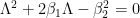
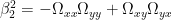
So Stability?

Let’s deal with the collinear points first because they make the math a bit easier. Because y is equal to zero, any terms multiplied by a y also go to zero which just leaves us with the following equations for β
$\beta_1 = 2-\frac{\Omega_{xx}+\Omega_{yy}}{2}$
$\beta_2^2 = -\Omega_{xx}\Omega_{yy}$
Solving the now simplified quadratic equations we see that the first Λ1 is positive and Λ2 is negative. This means that of our four roots, one is positive real, one is negative real, and two are purely imaginary. This means that all the collinear Lagrange points are unstable saddle points. In plain English, if we place any object close, but not perfectly on one of these Lagrange points the object will move away from the Lagrange point.

A Brief Aside About Space Stations

Whenever I talk about Lagrange points people ask me about space stations. From the High Frontier, to Journey to the Far Side of the Sun, to Another Earth, lots of science fiction authors, and some real scientists/engineers, have talked about putting space stations at various Lagrange points. As we just found out, these collinear Lagrange points are unstable. This means that any station would require continuous maneuvers to maintain it’s location. Still, missions like the James Webb Space Telescope and the NASA Lunar Gateway are being placed in orbits near unstable Lagrange points. I’m planning on getting to them in a future post where I talk only about missions near Lagrange points, but I wanted to build up the theory first. Once you understand the theory behind the Lagrange points, their stability, and nearby orbits; the reasons behind NASA’s current decisions become much clearer.

Equilateral Lagrange Points

So we’ve seen that the collinear Lagrange points are unstable, but what about equilateral Lagrange points? we can now use the nice short equations for their x and y positions that we found in the Lagrange points post

$x=\mu-\frac{1}{2}$
$y=\pm\frac{\sqrt{3}}{2}$
This simplifies our characteristic equation to
$\Lambda^2+\Lambda+\frac{27}{4}(1-\mu)$
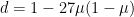
Because we know they appear in pairs, we also don’t really care what the eigenvalues are, just whether they are purely real or imaginary. For that we can look at the discriminant,d.
$d = 1-27\mu(1-\mu)$
if d is positive all the roots will be imaginary. If d is negative, then the roots will be a mixture of real, positive, and negative like with the collinear points. This means that if μ≤.03852 the motion around the L4/L5 Lagrange points are bounded, which is a really unexpected result! That means we can get orbits like this in the earth moon system

If μ≤.03852 we have two different imaginary roots. Each one of these roots correspond to a different period of oscillation. These two periods are, unsurprisingly, called the long and short period.

Theories Nice, but What About Reality?

So far we’ve been investigating the circular restricted three body problem, an idealized version of planetary motion. In our solar system there are more than 3 planets, and their orbits aren’t circular. Can we explain real world phenomena with such a restricted model?
Yes!
If we look at the figure below, we have a map of the solar system out till Jupiter with asteroids. I’ve added on a Sun-Jupiter coordinate system and marked down the rough locations of the L4/L5 Lagrange points.

You’ll notice that there are clumps of green dots around the L4/L5 points. These are called the Trojan asteroids.They behave almost exactly as predicted in the CR3BP. Jupiter has a μ of .00095 which fits into our theory exactly. Isn’t it nice when theory and reality line up ‽

Want more Gereshes

If you want to receive the weekly Gereshes blog post directly to your email every Monday morning, you can sign up for the newsletter here! Don’t want another email? That’s ok, Gereshes also has a twitter account and subreddit!

Stability of the Lagrange Points – Three Body Problem