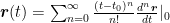
Lagrange F&G solution - The 2-Body Problem

Power Series Approximation

A Taylor series is a useful tool in analyzing functions. It allows us to break up those function into an infinitely long, easier to deal with, polynomial. The general formula of a Taylor series is, for some function r(t)

$\boldsymbol{r}(t)=\boldsymbol{r_0} + \frac{(t-t_0)}{1!}\frac{d\boldsymbol{r}}{dt}|_0 + \frac{(t-t_0)^2}{2!}\frac{d^2\boldsymbol{r}}{dt^2}|_0+...$

Note: The vertical line with a zero at the bottom means evaluate this function at 0, and the exclamation mark means factorial.

Now, this polynomial is infinite in length, so I’m going to rewrite it using summation notation

$\boldsymbol{r}(t) = \sum_{n=0}^{\infty}\frac{(t-t_0)^n}{n!} \frac{d^n\boldsymbol{r}}{dt}|_0$

In our case, that function we are approximating, r(t), is the radius vector. We have its derivative at time 0 because we have it’s initial velocity. Additionally, we have it’s acceleration at time 0, using newtons equation of gravitational attraction. Unfortunately we don’t have any higher ordered derivatives so we will need to derive them from the equation of motion, which is highly nonlinear.

Lagrange’s Fundamental Invariants

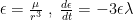
Lagrange put his mind to this problem and found that there were a set of three values that the derivative could always be expressed in. AKA, they form a closed set when differentiating the radius by time. These are ε,λ,ψ, and are called the fundamental invariant.

$\epsilon=\frac{\mu}{r^3} \;,\; \frac{d\epsilon}{dt}=-3\epsilon\lambda$

$\lambda=\frac{\boldsymbol{r}\bullet\boldsymbol{v}}{r^2}\;,\; \frac{d\lambda}{dt}=\psi-\epsilon-2\lambda^2$

$\psi=\frac{\boldsymbol{v}\bullet\boldsymbol{v}}{r^2}\;,\; \frac{d\epsilon}{dt}=-2\lambda (\epsilon + \psi)$

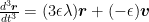
Now I’m going to write out the first few derivatives in terms of the fundamental invariant as well as the position and velocity vectors.

$\frac{d\boldsymbol{r}}{dt} =\boldsymbol{v}$

$\frac{d^2\boldsymbol{r}}{dt^2} =-\epsilon\boldsymbol{r}$

$\frac{d^3\boldsymbol{r}}{dt^3} =(3\epsilon\lambda)\boldsymbol{r}+(-\epsilon)\boldsymbol{v}$

$\frac{d^4\boldsymbol{r}}{dt^4} =(-15\epsilon\lambda^2 + 3\epsilon\psi - 2\epsilon^2)\boldsymbol{r}+(6\epsilon\lambda)\boldsymbol{v}$

$\frac{d^5\boldsymbol{r}}{dt^5} =(-105\epsilon\lambda^3 - 45\epsilon\psi\lambda + 30\epsilon^2\lambda)\boldsymbol{r}+(-45\epsilon\lambda^2+9\epsilon\psi-8\epsilon^2)\boldsymbol{v}$

We can continue on with his process for the rest of time, but I’ll stop here. Through rearranging this we can see that the position at any time can be represented by an equation of the form

$\boldsymbol{r}(t)=\boldsymbol{F}(t)\boldsymbol{r}_0+\boldsymbol{G}(t)\boldsymbol{v}_0$

A Hunt for an Exact Solution

Now to determine the F and G above, we have three choices. First, we could keep taking derivatives until we get to an approximation that is close enough to suit our needs. Second, we could look into seeing if there is a recursive equation for determining F and G so that we can calculate it until it converges, cutting out the derivative taking portion. Note there is a recursive formula but I’m skipping it here. If you are interested in it it is in Battin pages 112-114. Third, and finally, we can calculate exact values for F & G analytically. Let’s go with the third option.

Perifocal Coordinate System

Figure 1: The perifocal coordinate system, satellite in yellow

As we learned in an earlier post, all motion for the two body problem is in a single plane, the orbital plane. Let’s define a coordinate system for this plane, with the origin at the focus closes to the periapse of the orbit.

Now, let’s place our first axis from the origin to the periapsis of the orbit and we will denote this as i_e. Our second axis will go from the origin along the semilatus rectum in the positive direction, and be denoted i_p. The third vector, completing the triad, is parallel to the angular momentum of the object orbiting. In figure 1 we can see the perifocal coordinate system. f is the angle between i_e and the radius vector and is called the true anomaly.

Note: why did we call that first vector i_e? Because it points in the direction of the eccentricity vector. Semi latus rectum, Eccentricity vector are both terms from our contents of integration post and are showing up in extremely geometric ways for our orbit. Pause and ponder on why that is for a few moments.

Deriving the Exact Solution

Let’s express the radius and velocity equation in terms of the true anomaly, f

$\boldsymbol{r}=r\cos(f)\boldsymbol{i}_e+r\sin(f)\boldsymbol{i}_p$

$\boldsymbol{v}=-\frac{\mu}{h}\sin(f)\boldsymbol{i}_e+\frac{\mu}{h}(e+\cos(f))\boldsymbol{i}_p$

Now i_e and i_p are constant and can be expressed at any time if we know the radius, velocity, and true anomaly for any time. For simplicity lets say we know it at time 0.

$\boldsymbol{i}_e=\frac{\mu}{h^2}(e+\cos(f_0))\boldsymbol{r}_0-\frac{r_0}{h}\sin(f_0)\boldsymbol{v}_0$

$\boldsymbol{i}_p=\frac{\mu}{h^2}\sin(f_0)\boldsymbol{r}_0+\frac{r_0}{h}\cos(f_0)\boldsymbol{v}_0$

If we were to substitute these two last equations into our equations for relating radius and velocity we would get something of the form

$\boldsymbol{r}=\boldsymbol{F}_t\boldsymbol{r}_0+\boldsymbol{G}_t\boldsymbol{v}_0$

$\boldsymbol{v}=\boldsymbol{F}_t\boldsymbol{r}_0+\boldsymbol{G}_t\boldsymbol{v}_0$

How to use Lagrange F&G

If you know the initial position vector, the initial velocity vector, the initial true anomaly, you could propagate out the orbit to any true anomaly you wanted with the following procedure. First define the true anomaly difference

$\theta=f-f_0$

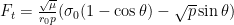
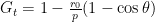
Then calculate

$\sigma_0=\frac{\boldsymbol{r}_0\bullet\boldsymbol{v}_0}{\sqrt{\mu}}$

Now pause and ponder, what quantity does σ represent? Is the zero subscript necessary?

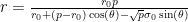
Once you are done pondering, calculate the current magnitude of position of the orbit using

$r = \frac{r_0p}{r_0+(p-r_0)\cos(\theta)-\sqrt{p}\sigma_0\sin(\theta)}$

Now that we have evaluated all the sub components, we can now calculate the Lagrangian coefficients using the following equations

$F = 1-\frac{r}{p}(1-\cos(\theta))$

$G = \frac{rr_0}{\sqrt{\mu p}}\sin(\theta)$

$F_t = \frac{\sqrt{\mu}}{r_0p}(\sigma_0(1-\cos\theta) - \sqrt{p}\sin\theta)$

$G_t = 1-\frac{r_0}{p}(1-\cos\theta)$

Code

I’ve put together a quick MatLab live script that implements the F&G solution that you can find here.

Perks of this Method over Forward Integration

You might ask, if we need the initial radius and velocity vector, why don’t we just integrate this equation forward in time using the governing equation? Numerical integration is more straightforward than our approach, and we can directly relate time, to position there?

Two reasons. The first is that when this method was created, computers were not yet around, so numerical integration was an extremely costly thing to do. Second, and the reason we went over it today, is because it lacks the compounding error present in forward integration. Because the F&G solution propagates the orbit from the initial velocity and position, the error from calculation, and mis-measurement of initial conditions stays constant through your propagated orbit. With numerical integration, any error from calculating the last position, is carried over into the next calculation. This error can build over time and the longer you continue on, the worse this error can get.

Want More Gereshes…

If you want to receive the weekly Gereshes blog post directly to your email every Monday morning you can sign up for the newsletter here!

If you can’t wait for next weeks post and want some more Gereshes I suggest

Undergraduate Engineering EDC

Rollout of a rocket motor test stand

What is the n-Body Problem?

Lagrange F&G solution – The 2-Body Problem