Verlet Integration - The n-Body Problem

Review of the n-body Problem

The n-body problem is when some number of bodies are interacting with each other gravitationally, and you want to figure out what their movement will be at some arbitrary point in the future. I wrote a full post on the problem and it’s difficulties here. I highly recommend that post as it contains some of my favorite graphics, including this series of relative views of the same 8-body simulation

The gravitational force on a body caused by another body can be found through Newton’s law of gravitational attraction.

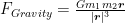
$F_{Gravity}=\frac{Gm_1m_2\boldsymbol{r}}{|\boldsymbol{r}|^3}$

where G is the universal gravitational constant, m is the masses, and r is the vector of relative displacement between the two bodies. Each body produces a force on every other body. You should also note the denominator of the right-hand side. Those two raised bars signify a vector norm (2-norm). Because of the norm being raised to the third power, this equation is nonlinear. Also, note there’s a singularity in the equation.

Once we know all the forces on a specific body, we can appeal to Newton’s second law to find it’s acceleration

$m\ddot{\boldsymbol{X}}=\sum_{i=1}^nF_i$

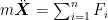
We’ll end up with n governing equations in each dimension. Because of that nonlinearity, I mentioned earlier, there is no general closed-form solution when the number of bodies you are analyzing is 3 or larger. I flew through that explanation of the n-body problem so if you want to get a little more information I’ll again link to my past post which dives deeper on what is the n-body problem.

What is Verlet Integration?

Because the equations of motion in the n-body problem are nonlinear and cannot be solved through analytical integration, let’s turn to a numerical method. We want to find the position of a planet sometime in the future given we know their initial conditions and the equations of motion.

Let’s take a step back from the flawed world of dynamics and to the perfect world of kinematics. Here, the integral of acceleration is always velocity whose integral is always position. If we knew the initial position, and velocity as well as the infinite number of derivatives, and then we integrated each one to get their contribution to position, we could know the position at any time. Representing this as an equation we would get the following

$x(t)=x_0+v(t)t+\frac{a(t)t^2}{2}+\frac{j(t)t^3}{6}+...$

j is the jerk, which is just the derivative of acceleration. After jerk, there are the higher derivatives like jounce but when dealing with classical mechanics there are zero forces associated with derivatives higher than acceleration. Fun comedic names are often given to these derivatives like snap, crackle, and pop.

Lets now nudge this equation both forward in time and backwards in time by some small Δt

$x(t+\Delta t)=x(t)+v(t)\Delta t+\frac{a(t)\Delta t^2}{2}+\frac{j(t)\Delta t^3}{6}+O(\Delta t^4)...$

$x(t-\Delta t)=x(t)-v(t)\Delta t+\frac{a(t)\Delta t^2}{2}-\frac{j(t)\Delta t^3}{6}+O(\Delta t^4)...$

and now let’s add them together

$x(t+\Delta t)+x(t-\Delta t)= 2x(t)+a(t)\Delta t^2+O(\Delta t^4)$

and do some algebra

$x(t+\Delta t) = 2x(t)-x(t-\Delta t)+a(t)\Delta t^2+O(\Delta t^4)$

We now have an equation for stepping forward the equation in time provided we know it’s current acceleration, current position, and last position.

Note on that Big O at the End

You may have noticed that big O(Δt) appeared at the end of several of the above equations appearing after the jerk term. If I were to cut it off, set it equal to some variable y, and place it below what would you think it is?

$y=O(\Delta t^4)$

If you thought of a function of t to the fourth power you would be right. What we did was take all the terms larger than jerk and lumped them into this function O(Δt)

$O(\Delta t^4) =\frac{x^4(t)\Delta t^4}{4!}+\frac{x^5(t)\Delta t^5}{5!}+\frac{x^6(t)\Delta t^6}{6!}+...$

Why is the O(Δt) function only to the fourth power? In the above equation, there are higher powered terms. We want to be able to ignore these terms. If Δt is less than one than taking Δt to some power makes it go towards zero. the higher the power the faster it goes towards zero. Out of all the infinite remaining terms that we lumped into O(Δt), the one that will contribute the largest error is the first term that goes to the fourth power. We leave the to the fourth power in the O(Δt) so that when we take a look at the error from truncating the last term we know that it changes quarticly with Δt.

Example Time!

Now that we know what Verlet integration is, let’s see how it stacks up against a first order FOrward Euler (FOE) integration. Note if you want to learn more about forward Euler implementations, I go over it in my post on modeling fireflies in sync.

Let’s see how both do when integrating a 5-body system forward in time with the same initial conditions. First up the Verlet integrator

Now let’s see how the FOE integrator did

Wait a minute. Those don’t even look similar, what happened? I’ll go over that in the next section, but take a few minutes to pause and ponder what might have happened. I can tell you that the initial conditions and governing equations are exactly the same.

Note: You can find the code that produced these plots here. Running that script will produce different plots than above because a new set of initial conditions are generated randomly every time you run it.

Pause and Ponder

So now that you’ve hopefully taken a few minutes to think about what went happened let’s go over it. If we plot the difference between the two integrators in the x and y position over time we get the following plot.

We can see that the error begins at 0 and then diverges relatively constantly as time increases. We can attribute this divergence to two factors, the difference between the integrators, and the choice of model.

Differences Between the Integrators

There are tons of different numerical integration schemes, each with their own benefits and drawbacks. Some are extremely quick and lightweight, while others are good at handling nonlinearities. The Verlet integrator was designed to integrate newtons equations of motion. It’s a relatively simple to compute integration scheme and has a quartic error with the step size you’re taking. The FOE integrator used in this post is also extremely simple but has an error that’s quadratic with step size. This means that the step size for a FOE needs to be the square root of the step size of a verlet integrator to get the same accuracy. Because the last steps results are used to calculate the current step’s results, the error compounds over time and the two integrators diverge.

Choice of Model

The choice of model also played into how the model diverged. If we were modeling a pendulum swinging, the error in angle would be bounded to twice the initial angle. A pendulum is a marginally stable system, and while there will be an error between the two integrators it wouldn’t contentiously increase. If we added friction to our pendulum, to make it a stable system, then the error between the two integrators would decrease to zero after a large enough period of time.

Unlike the pendulum example above, the n-body problem is not inherently stable. This means that the difference between the two integrators is unbounded and can grow to an infinitely large size. Additionally, when you are dealing with 3 or more bodies, the system is chaotic. This means the system is extremely sensitive to small changes between the two integrators.

Note: a big misconception that some people have is that chaotic means stochastic, it does not. Chaotic systems without random elements are deterministic. I’ll talk more about chaotic systems and misconceptions people have about them in a future post because this post is already too long.

So which integrator did better? The verlet integrator by a mile.

Why Such a Bad Match-up

You might think to yourself why did I choose the FOE integrator if I knew it would have so much more error then the verlet model and the system was extremely sensitive to error? Because I wanted to highlight how much better the verlet model is in certain scenarios and also show how you need to be cognizant of whichever integration scheme you are using. Different integration schemes have different benefits and we must know the strengths and weaknesses of the scheme before we use it. Using schemes blindly and without a a knowledge of the assumptions made is one of the quickest ways to something going wrong.

Why Euler/RK methods are used more often

Now that we’ve seen how the Verlet integration scheme outperform a FOE scheme, why would we ever want to use an Euler method? Because it’s much more general. An Euler method can be used in case where we aren’t looking at newtons equations of motion. If we wanted to go back to the classic ODE example of modeling fox and rabbit populations we couldn’t use verlet integration but a FOE scheme with a suitable time step would work just fine. There are also ways to extend Euler’s method to higher orders called Runge-Kutta methods and ways to make it adaptively time step which is what MatLab’s ODE45 does. Different schemes allow you to handle stiff equations well and others can take sharp nonlinearities into account. A good beginning overview of different numerical methods for solving differential equations can be found here.

Note this post was inspired by two of LeiosOS’s videos on FOE, and Verlet integration. He has a great channel and you should check him out!

Want More Gereshes?

If you want to receive the weekly Gereshes blog post directly to your email every Monday morning you can sign up for the newsletter here!

If you can’t wait for next weeks post and want some more Gereshes I suggest

Undergraduate Engineering EDC

Rollout of a rocket motor test stand

What is the n-Body Problem?

Verlet Integration – The n-Body Problem