Preliminary Orbit Determination

What is Orbit Determination

When we are dealing with two bodies, we can determine their orbital paths exactly using a certain set of orbital elements. If you want to learn more about these orbital elements you can find my post on them here and how to use them to determine an orbital path here. If we have a certain set of orbital elements, assuming Keplerian motion, we can tell where the satellite was, is, and will be for all time. But what if we don’t have those orbital elements? That’s where orbit determination comes in.

First, let’s think of some cases where we wouldn’t have direct knowledge of the orbital elements. One case would be if our rocket had a malfunction and placed our satellite in the wrong orbit. Another would be if we were trying to track another countries spy satellite. A historical need for orbit determination, and one that let many of the earliest mathematical advances, was trying to determine the orbits of the other planets in our solar system.

Orbit Determination is a Big Topic

Now that we know there are many uses, both for past and present problems, is there one correct way to do orbit determination? No.

There are hundreds of different orbit determination schemes. They differ based on the necessary inputs, the constraints of the problem, and the solving accuracy they provide. I could spend the next year just wring posts on orbit determination. Comparing and contrasting the different methods, deriving some, leaving others as vague ideas, and still have topics to talk about. It’s a large topic and the rest of this post will only scratch the surface of three extremely basic methods.

The three methods I’m highlighting are from section 3.7 of Battin’s Introduction to Astrodynamics.

Orbits from 3 Co-planar Positions

The first of the three methods requires us to have 3 co-planar position measurements in polar coordinates. That means we have r1,θ1,r2,θ2,r3, and θ3. We return to our equation of orbit we found in a prior post which is.

$r=\frac{p}{1 + e\cos(\theta-\omega)}$

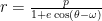
where

$\theta = \omega + f$

By appealing to angle difference identities we can transform our equation of orbit to the following

$r=\frac{p}{1+e\cos(\theta)\cos(\omega)+e\sin(\theta)\sin(\omega)}$

Let’s now introduce two variables P and Q that are defined as

$P=e\cos(\omega)$

$Q=e\sin(\omega)$

Which lets us linearize our equation of orbit with

$r=\frac{p}{1+\cos(\theta)P+e\sin(\theta)Q}$

Through some algebraic manipulation we get the following

$\frac{p}{r_n}-P\cos(\theta_n)-Q\sin(\theta_n)=1$

We have 3 unknowns in the above equation, p,P, and Q. This is why we need 3 different measurements. 3 equations, 3 unknowns, I leave determining the values for p,P, and Q up to a suitable method of your choosing. Once you have these three determining the eccentricity and ω are trivial. Hint think of using trig identities and come out with the following.

$e=\sqrt{P^2+Q^2}$

$\tan(\omega)=\frac{Q}{P}$

Orbit Determination with 3 Position Vectors (Gibb’s Method)

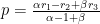
Before we began with 3 co-planar positions. But what if we are not in the same orbital plane as the object we are observing? This method is like the last method, just with vector algebra. Here, we have 3 position vectors, r1,r2, and r3. Because we are dealing with Keplerian orbits, those 3 measurements can be assumed to be to co-planar points. First calculate alpha and beta

$\alpha=\frac{\boldsymbol{r}_2\times\boldsymbol{r}_3\bullet\boldsymbol{n}}{n^2}$

and

$\beta=\frac{\boldsymbol{r}_1\times\boldsymbol{r}_2\bullet\boldsymbol{n}}{n^2}$

where n is defined as

$\boldsymbol{n}=\boldsymbol{r}_1\times\boldsymbol{r}_3$

We can now find the semi-latus rectum, p, using the following equation

$p = \frac{\alpha r_1 - r_2 + \beta r_3}{\alpha -1+\beta}$

Now in order to find the eccentricity lets take the cross product of n and e

$\boldsymbol{n}\times\boldsymbol{e}=(p-r_1)\boldsymbol{r}_3-(p-r_3)\boldsymbol{r}_1$

Because we also know that e is normal to n we have the following relationship

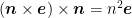
$(\boldsymbol{n}\times\boldsymbol{e})\times\boldsymbol{n}=n^2\boldsymbol{e}$

Combining these last two relations we get

$n^2\boldsymbol{e} = [(p-r_1)\boldsymbol{r}_3\times\boldsymbol{n}] - [(p-r_3)\boldsymbol{r}_1\times\boldsymbol{n}]$

This is known as Gibb’s method and is often used as an initial orbit determination method. Once you know the rough orbital elements you can narrow down your solution space and use this as your initial estimate in more powerful iterative orbit determination algorithms.

Approximate Orbit from Three Position Fixes

While the above two methods will give us the exact orbital elements if we have perfect inputs, they both fall victim to increased numerical errors durring calculation if the angles between the measurements are small. Because we’ve only been looking at 3 position vectors, we have been using geometry to determine the orbital elements. If we begin to also record the times at which we take our measurements, we can also use our understandings of the dynamics of the system to improve our estimates of the system.

Now lets say we have measurement vectors r1,r2,r3 and the time of respective measurement t1,t2,and t3. These 6 pieces of information can be related by a fifth order power series expansion.

$\boldsymbol{r}=\boldsymbol{a}_0+t\boldsymbol{a}_1+t^2\boldsymbol{a}_2+t^3\boldsymbol{a}_3+t^4\boldsymbol{a}_4+t^5\boldsymbol{a}_5$

Take it’s derivative to get

$\boldsymbol{v}=\boldsymbol{a}_1+2t\boldsymbol{a}_2+3t^2\boldsymbol{a}_3+4t^3\boldsymbol{a}_4+5t^4\boldsymbol{a}_5$

one more derivative where A is acceleration

$\boldsymbol{A}=\frac{-\mu}{r^3}\boldsymbol{r}=2\boldsymbol{a}_2+6t^1\boldsymbol{a}_3+12t^2\boldsymbol{a}_4+20t^3\boldsymbol{a}_5$

Note that we had 6 pieces of information and we now have 6 unknown coefficients from a0 to a5.

Let’s also define a set of time intervals just to make our equations a bit tidier

$\tau_1=t_3-t_2 \quad \tau_2=t_3-t_1 \quad \tau_3=t_2-t_1$

Now, I’m going to give you the next step and it might not be obvious where we are going with this so take a moment to stop and think about what it looks like we’re doing. replace t in the power series successively by -τ3,0, and τ1. You should get the following 7 equations.

$\boldsymbol{r}_1=\boldsymbol{a}_0-\tau_3\boldsymbol{a}_1+\tau_3^2\boldsymbol{a}_2-\tau_3^3\boldsymbol{a}_3+\tau_3^4\boldsymbol{a}_4-\tau_3^5\boldsymbol{a}_5$

$\boldsymbol{r}_2=\boldsymbol{a}_0$

$\boldsymbol{r}_3=\boldsymbol{a}_0+\tau_1\boldsymbol{a}_1+\tau_1^2\boldsymbol{a}_2+\tau_1^3\boldsymbol{a}_3+\tau_1^4\boldsymbol{a}_4+\tau_1^5\boldsymbol{a}_5$

$\boldsymbol{v}_2=\boldsymbol{a}_1$

$\frac{-\mu}{r_1^3}\boldsymbol{r}_1=2\boldsymbol{a}_2-6\tau_3^1\boldsymbol{a}_3+12\tau_3^2\boldsymbol{a}_4-20\tau_3^3\boldsymbol{a}_5$

$\frac{-\mu}{r_3^3}\boldsymbol{r}_3= 2\boldsymbol{a}_2$

$\frac{-\mu}{r_3^3}\boldsymbol{r}_3=2\boldsymbol{a}_2+6\tau_1^1\boldsymbol{a}_3+12\tau_1^2\boldsymbol{a}_4+20\tau_1^3\boldsymbol{a}_5$

Note: It reminded me of taking a finite difference. Namely a central difference. We’re finding the velocity at the second point by using the time it took to go from the first point to the third point and incorporating the system dynamics.

If we solve this system of equations for v2 we get the following

$A_0\boldsymbol{v}_2=A_1\boldsymbol{r}_1+A_2\boldsymbol{r}_2+A_3\boldsymbol{r}_3$

$A_0=12\tau_1\tau_2\tau_3(\tau_3-\tau_1)(2\tau_1^2+5\tau_1\tau_3+2\tau_3^2)$

$A_1=\tau_1^4[12(2\tau_2+3\tau_3)+\frac{\mu\tau_3^2}{r_1^3}(\tau_1+3\tau_2)]$

$A_2=\frac{\mu}{r_2^3}\tau_1^2\tau_2\tau_3^2(8\tau_2^2+3\tau_1\tau_3)-12\tau_2[2\tau_2^4-5\tau_1\tau_3(\tau_2^2+\tau_1\tau_3)]$

$A_3=\tau_3^4[12(3\tau_1+2\tau_2)+\frac{\mu}{r_3^3}\tau_1^2(3\tau_2+\tau_3)]$

Now, this looks promising. We get v2 and by combining that with r2 we can pull out the orbital elements in the classical way. Unfortunately, this solution happens to have a problem. It doesn’t work when τ1 = τ3. Try plugging those in and see what you get! This means that we cant use this method with regularly spaced measurements. Additionally because we live in the real world of numerical accuracy, any measurements that are nearly regularly spaced will suffer from large computational error. I haven’t done a sensitivity analysis but I would expect this error to grow exponentially as we get closer to regularly spaced measurements.

Luckily for us, Samuel Herrick determined a work around. This article is already quire long so I will just present it here and leave the derivation to the determined reader (The skeleton of the derivation is presented on Page 135 of Battin’s Intro to Astrodynamics if you get stuck).

$\boldsymbol{v}_2=-\tau_1(\frac{1}{\tau_2\tau_3}+\frac{\mu}-{12r_1^3})\boldsymbol{r}_1-(\tau_3-\tau_1)(\frac{1}{\tau_1\tau_3}+\frac{\mu}{12r_2^3})\boldsymbol{r}_2+\tau_3(\frac{1}{\tau_1\tau_2}+\frac{\mu}{12r_3^3})\boldsymbol{r}_3$

Again once we have v2 we can use it with r2 to determine the orbital elements using formulas we derived here.

How we get these Measurements?

Radar stations on the ground obtaining the position vectors of a satellite in orbit

Much like how this post is a very basic introduction to orbit determination, I will only briefly be covering the most common way of how we get these measurements from Earth-based observatories. We can ping the satellite with an electromagnetic wave and measure how long it takes to get there and come back. We can estimate the velocity of the signal in the earth’s atmosphere and the vacuum of space so we can figure out the range rather well. If we have two ground stations that receive the same message, we can determine the satellites relative location by looking at the difference in the ping’s time of flight. When done with a laser this is called laser range-finding and when done with radio waves it’s called radar.

Want more Gerehses…

If you want to receive the weekly Gereshes blog post directly to your email every Monday morning you can sign up for the newsletter here!

If you can’t wait for next weeks post and want some more Gereshes I suggest

Undergraduate Engineering EDC

Rollout of a rocket motor test stand

What is the n-Body Problem?

Preliminary Orbit Determination – 2-Body Problem