Chaotic Swirls and the Duffing Equation

Springs, Except More Fun

In any introductory physics or differential equation’s class we are introduced to the simple spring mass system. Because of Hooks law it’s nice, linear, and easy to analyze. But not all springs follow Hooks Law. Some, like the duffing spring we’ll analyze in this post, are nonlinear and chaotic.

What’s a Duffing Spring?

A normal spring produced a force that’s linearly proportional to the amount it’s stretched out. This is called Hook’s law and is represented as

$F_{Hooks}=-Kx$

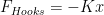
Where K is a constant and x is the displacement of the spring. A duffing spring is one where the force is represented as

$F_{duff}= -ax - bx^3$

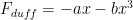
where a and b are constants. This changes the equations of motion for a driven spring mass system to be

$\ddot{x} + \delta\dot{x} + ax +bx^3 = \gamma\cos(\omega t)$

Let’s look at what the different constants do

ω is the frequency that the system is being driven at
γ is the maximum force driving the system
b is the nonlinear “stiffness” of the duffing spring
a is the linear stiffness of the spring
δ is the dampening present in the system

The addition of the cubic term to the equations of motion has changed the system from a nice and easy to analyze linear system to a non-linear and chaotic system.

Chaotic?

You might be asking yourself

How can it be chaotic? It only has two dimensions, don’t you need a minimum of 3 dimensions for it to be chaotic?

Stroatz’s Nonlinear Dynamics and Chaos goes over this more, but we can consider time to be the third dimension with a differential equation of

$\dot{t}=1$

Phase Space

As we change the parameters, we can get different results. Let’s set all the parameters to be a constant except for γ. We’ll vary γ and see how it changes in both the time domain and the phase space.

On the left of the graph we have the position as a function of time. A pretty standard display. On the right of the graph we have a phase portrait. Phase portraits are when we plot the states against each other instead of time. The really interesting thing about the duffing spring is that as we increase γ we go from a periodic trajectory to a chaotic trajectory. This is where the graph begins to jump around; small changes to γ result in large changes in the trajectory. But the chaos doesn’t continue forever. The duffing spring settles back down on a more complex, but very periodic motion after a while and stays there through a reasonable range of γ. After this oasis of calm periodic behavior we once again return to the chaotic dynamics. I only plotted γ for a small range ( between .25 and .55) but if we continued it farther it would continue to show it switching between chaotic and periodic regions which is quite cool.

Note: all of these trajectories began with the same initial conditions, but I waited until their transient behavior died down to plot the trajectory.

Transform!

We have 5 different parameters we can play with in the way we set up the equations of motion. Is there anyway to reduce this? Yes!

Let’s apply the following transformations

$\tau = t\sqrt{a}$

$y = \frac{xa}{\gamma}$

This converts our equation of motion into

$\ddot{y}+2\eta\dot{y}+y+\epsilon y^3 = \cos(\sigma\tau)$

where the new parameters are defined as

$\eta = \frac{\delta}{2\sqrt{a}}$

$\epsilon = \frac{b \gamma^2}{a^3}$

$\sigma = \frac{\omega}{\sqrt{a}}$

This transformation is useful because we’ve compressed the information needed to describe the system into 3 parameters instead of 5. Note: for this transformation to work, we would need a to be greater then zero. This is ok because that means our dampener removes energy from a system like most real world dampeners do.

Poincare Section

I plan to do a whole post about Poincare sections, but for now think of them as tools to reduce the dimension of the system and visualize periodic and quasi-periodic orbits. I’ve plotted the Poincare section of the duffing spring below where I sweep through different times.

Plotting the Poincare section is usually one of the easiest ways to find a fractal in a chaotic system, and the duffing spring is no exception. This fractal has a dimension of about 1.3. What’s more, this fractal we’ve plotted is the duffing spring’s chaotic attractor.

Want more Gereshes

If you want to receive the weekly Gereshes blog post directly to your email every Monday morning, you can sign up for the newsletter here! Don’t want another email? That’s ok, Gereshes also has a twitter account and subreddit!