

Disclaimer: Plotly paid me to both make a dash app, as well as this post. Even before this I was a fan of Plotly’s products and used them in posts about missed thrust events and visualizing periodic orbits. In those projects, I used Plotly because they make some great visualization tools. You should check their stuff out.
Landing a Lunar Lander without a Gimballing Engine
When the Apollo Lunar Module landed on the moon, it oriented itself using a reaction control system made up of small thrusters located about the lander. The main engine, located at the bottom, was fixed in place and only used to slow the spacecraft down. This restriction makes designing a lunar landing trajectory more difficult, so let’s explore the trade space of optimal control trajectories. Note: If you want to try the interactive Dash app directly, without going through all the math, you can find that here.
If we restrict it to 2 dimensions, we would obtain the following equations of motion


In these equations of motion, which come from this paper, where u is the spacecraft’s thrust fraction, B is its pitch rate, c1 its max thrust, c2 the engines efficinecy, and c3 its max pitch rate.
Solving the Optimal Control Problem using Casadei
We’re going to solve two separate optimal control problems in this post, a mass optimal control problem, given by the following equation

and a time otpimal control function

In order to solve the optimal control problem, we are going to use a direct method, which we’ve discussed generally here.
In this problem we’re going to have the following boundary conditions


and

with the exception of the final mass and final time, which we’re going to leave free. We’re going to enforce the following path constraints

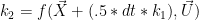
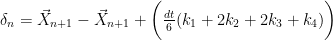
as well as a one-step Runge-Kutta 4 constraint on the dynamics


Now that we have turned our out optimal control problem into a nonlinear programming, we are going to use CasADi, an “open-source tool for nonlinear optimization”. Here’s a good tutorial about how to use CasADI
Exploring the trade space with a dash app
Instead of exploring the tradespace through images I encourage you to interact with the dash app yourself, you can find it here with the source code here.
Places to learn more about dash apps
If you want to learn more about Dash apps, this is a great resource for getting started, and there’s a forum that I went to for more advanced questions.
Additionally, if you want to see some other creative uses of Dash, they have a Dash gallery.
Want More Gereshes?
If you want to receive the weekly Gereshes blog post directly to your email every Monday morning, you can sign up for the newsletter here! Don’t want another email? That’s ok, Gereshes also has a twitter account and subreddit!