

Note: This post is adapted from a lecture I gave to my undergrads. It’s focused on conveying the method and main idea behind the different formulations. This is not a rigorous treatment and in some locations, I have traded being technically correct for being clear. If you want a riggorous treatment of the material I suggest a textbook.
Newtonian Mechanics
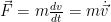
Newtons second law in mathematical form is
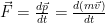
which states that the force is equal to the change in linear velocity (Note: this only holds in inertial reference frames). If mass is a constant then we can take it out of the derivative to obtain the familiar
Lagrangian Mechanics
Newtonian mechanics is a great starting point for many problems and lends itself well to simple problems that can be expressed in a Cartesian form. But what if cartesian coordinates are not the most natural for a specific problem? You can still use Newtonian mechanics, but you’ll find yourself knee deep in transformation matrices. Picture a two element a robot arm.
(insert picture of robot arm)
You can describe this system with the Cartesian coordinate of every joint, but that would be tedious. Your first instinct would be to instead describe this system with the angle at every joint, and this is the idea behind Lagrangian mechanics, that through judicious selection of our coordinate systems we can make our lives easier. Restating that formally; Lagrangian mechanics is a reformulation of Newtonian mechanics that makes using mixed coordinate systems easier. Let’s first define the Lagrangian, L, as
L = T – V
where T is the total kinetic energy of the system, and V is the potential energy of the system. The system can then be described by j independent coordinates, which are labeled
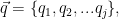
and their time derivatives, which are labeled

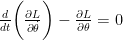
for a total of 2j states. We can then obtain the equations of motion through

We obtain this equation from the principle of least action, which in short says that if something happens in nature, it occurs along the path that minimizes the [energy]*[time] or the [momentum]*[distance]. Think about dropping a ball at rest from your hand, it will fall straight down. It will not first head up or create any intricate paths on it’s way down because any other path would increase the trajectories time/distance or momentum/energy. Nature always chooses the lowest stable energy configuration. If you want to see the derivation of this equation search “Euler-Lagrange derivation”.
Hamiltonian Mechanics
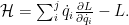
If the though behind Lagrangian mechanics is that the dynamics can best be expressed through a generalized set of coordinates and velocities, the thought behind Hamiltonian mechanics is, what if the dynamics can best be expressed through a generalized set of coordinates and momenta. If we could find just the right coordinates and momenta then the equations of motion of the system boil down to
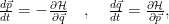
where 

and

Are these it?
Although these are the three most common formulations of mechanics, and the only ones covered here there are also
- Routhian Mechanics – Uses generalized velocities and generalized momenta (useful for cyclic coordinates)
- Apellian Mechanics – Useful when non-holonomic constraints are involved. (Derived through Gauss’s principal of least constraint instead of the principal of least action)
- Koopmanian/Neumannian Mechanics – Re-formulated classical mechanics into a quantum mechanical form
You can generally ignore these formulations though.
Reasons to use each
Newtonian mechanics
- Pro – Can easily handle dissipate forces like friction and drag (Called non-holonomic constraints)
- Pro – Can easily handle additional, non-potentiality forces
- Con – Derivation grows exponentially more difficult as constraints are added.
Lagrangian Mechanics
- Pro – Can easily handle constraints (that don’t do work)
- Con – Does not do well with dissipate forces like friction and drag
Hamiltonian Mechanics
- Pro – Very good for numerical integration
- Meh – Algebra is in obtaining the generalized momenta and Hamiltonian, not in obtaining the equations of motion
- Con – Non-intuitive
- Con – Does not do well with dissipate forces like friction and drag
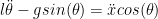
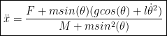
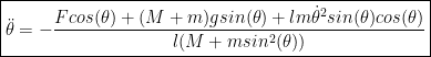
Worked Example – Pendulum on a Cart


If you want to see how we can control the cartpole, I recomend this post.
Want More Gereshes?
If you want to receive the weekly Gereshes blog post directly to your email every Monday morning, you can sign up for the newsletter here! Don’t want another email? That’s ok, Gereshes also has a twitter account and subreddit!