

Chaos
I’ve recreated one of my favorite mathematical demonstrations below. Three double pendulums, all starting with near identical initial conditions, all rapidly diverging. I love this demonstration because it’s such a great example of chaotic dynamics.

What is Chaos?
Chaotic dynamics, in a nutshell, means that a system is extremely sensitive to initial conditions. That means a small change in where the system begins, becomes a big difference in where it ends up. A lot of people say that chaos means that we cant predict what the system will do, and this is not exactly true. Chaotic systems, including the one we are looking at today, can be deterministic. This means that if we know it’s initial conditions, and can integrate it forward in time with infinite precision, we could predict its motion out arbitrarily into the future. Unfortunately, in the real world, there’s always some measurement error in determining the initial conditions and computers only have finite precision. This means that in reality we often cant predict chaotic systems out arbitrarily into the future.
A more full explanation in chaos, cannot be completed without talking about bifurcations and fractals, so I will leave that to another post. If you want to read more about it on your own, I highly recommend Nonlinear Dynamics and Chaos by Strogatz.
Double Pendulum Equations of Motion
Finding the equations of motion for the double pendulum would require an extremely long post, so I’m just going to briefly go over the main steps. You can find a more complete walk-through here.

Unlike our normal approach of appealing to Newton’s second law, we are going to use the Hamiltonian reformulation of classical mechanics. We begin by finding the potential energy, V, of the system.

Next up we find the kinetic energy, T, of the system

We then get the Lagrangian, L by

We could use Euler-Lagrange equations to find the equations of motion, but I prefer using the Hamiltonian. To do this we first need to compute the generalized momenta. Our system has 2 degrees of freedom so we get two generalized momenta


The Hamiltonian is then given by
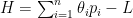
We can now use Hamilton equations to get the equations of motion
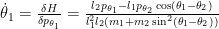
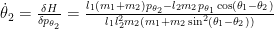


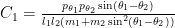
Note: C1 and C2 are just broken off to make writing the equations of motion more convenient.

Lissajous Appearum
We’ve seen the chaotic nature of the pendulums evolve, and derived their equations of motion. Now let’s see what structure we can tease out of plots.
Let’s give the pendulum a small initial displacement and plot the two pendulum angles as we watch it evolve.

It traces out the familiar form of a Lissajous curve. This small motion is highly regular and structured, why? Let’s turn to the small angle approximation. The small angle approximation means that when θ1 and θ2 are small, we can approximate their sin() and cos() as θ and 1 respectively. Additionally, because their momenta will be small (less than 1), the product of their momenta will be very small and can be ignored. this converts the nonlinear systems of equations into a nice set of linear ones. A good exercise for the reader would be to apply the small angle approximation to the equations of motion. If you look at the small angle equations of motion long enough they begin to look familiar. Almost like the system of equations for two masses connected by a spring.
Now what happens if we push the initial θ1 and θ2 far enough that the small angle approximation breaks down?

Both initial angles in the GIF above are .7 radians, which is about 40 degrees. This is outside the range of where the small angle approximation holds, but the small angle approximation isn’t binary. It doesn’t stop working after a certain angle. It slowly gets worse, and that’s what we see here. Instead of the nice rectangular Lissajous curve, we now get a Lissajous curve that’s been stretched and bent. It’s easy to see our trajectory is still bounded, but we have a much more complex nonlinear shape.
What if now we increases the initial angles to be much larger than the small angle approximation bounds?

We see the nonlinear dynamics in full effect with it’s wild trajectory. Note: I’ve chosen not to regularize the angles to remain between 0 and 2π because it doesn’t add additional structure and I liked the visual of the thetas walking around.
Want more Gerehses …
If you want to receive the weekly Gereshes blog post directly to your email every Monday morning, you can sign up for the newsletter here! Don’t want another email? That’s ok, Gereshes also has a twitter account and subreddit!
If you can’t wait for next weeks post and want some more Gereshes I suggest