Lyapunov Orbits

Everything Orbits About Something

In our solar system, Moons orbit around planets, which themselves orbit around the sun. Well, actual they orbit about the system barycenter, the combined center of mass between the two bodies. But can we get an object to orbit around a region without a barycenter? Yes! (Kinda) There are actually a few different types of these orbits, from Halo Orbits to Lissajous Orbits, but in this post, I’ll be going over the simplest type Lyapunov Orbits.

Note: this is an ongoing series on the CR3BP. If you want to get ahead on your own these are some good books on the material and astrodynamics in general (Book 1, Book 2, Book 3, Book 4).

Lagrange Points

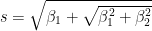
Before we get started on orbits, let’s first return to Lagrange points. These are the 5 points that stay stationary relative to the two major bodies in the CR3BP. I go over them in more detail here, but when we were analyzing the collinear points L1, L2, and L3 we found that each one had 4 eigenvalues, λi. One positive, one negative, and two imaginary. The single positive eigenvalue is enough to know the points are unstable, but the two imaginary values point to the possibility of a periodic orbit. In the linear region near the Lagrange points we can appeal to LTI Dynamics system theory and we know that a solution to the differential equation is

$x_{linear}=A_1e^{\lambda_1 t}+A_2e^{\lambda_2 t}+ A_3\sin(\lambda_3 t)+A_4\cos(\lambda_3 t)$

$y_{linear}=B_1e^{\lambda_1 t}+B_2e^{\lambda_2 t}+ B_3\sin(\lambda_3 t)+B_4\cos(\lambda_3 t)$

Where the Ai and Bi are determined by the initial conditions. The first two terms in each equation are the unstable and stable terms, so is there a way we can get rid of them? In other words, can we find some set of initial conditions to make A1, A2, B1, and B2 equal to zero?

Yes. It involves the following relationships,

$B_i = \nu_i A_i$

$\nu_i = \frac{\lambda_i^2-\Omega_{xx}}{2\lambda_i}$

but I’ll leave the algebraic manipulation up to you the reader. Instead I’ll skip to the end where if we have an initial x position we can get a y velocity that ensures A1, A2, B1, and B2 are equal to zero. Note: for this solution the y position and x velocity are both zero.

$s=\sqrt{\beta_1+\sqrt{\beta_1^2+\beta_2^2}}$

$\beta_3 = \frac{s^2+\Omega_{xx}}{2s}$

$\dot{y}_0 = -x_{pert 0}\beta_3 s$

Linear to Nonlinear

So now that we have found a linear periodic solution around L1, how good is it once we apply those same initial conditions to our completely nonlinear equations of motion?

The nonlinearities turn our nice linear periodic orbit into a non-periodic one. Before we get a periodic orbit in the non-linear problem let’s first take a sidebar to the mirror theorem.

Mirror Theorem

If we were to have some test point (x1,y1,z1,…) above the x-axis (y=0) and a corresponding one below the x-Axis (x1,-y1,z1,…) their x and z accelerations would be the same, but the y acceleration would be opposite (Easy enough for the reader to prove, just plug in the above test points to the EOM). A repercussion of this idea is that a particle that perpendicularly crosses the x axis twice (in two crossings) will be a periodic orbit.

Return to Dynamics

If we take the Mirror theorem along with our linear initial conditions, we already have one perpendicular crossing of the y-axis. How can we get another? Let’s once again see how our linear IC’s perform in the nonlinear dynamics model, but this time let’s only plot them until it crosses the x-axis.

Now our final state is not perpendicular but close to it. We can now use a shooting scheme to drive our final state towards a perpendicular crossing of the x-axis which would have the final states.

$\dot{x} = 0$

$y=0$

and we can adjust the time we are integrating for as well as our initial y velocity or x-position.

Now let’s integrate our full initial conditions out for a full orbit

As you increase the radius of the Lyapunov orbit, they become more kideny bean shaped

A Big Happy Family

There’s not just a single Lyapunov orbit, there’s a whole family of them. If we grow the L1 Lyapunov orbits out we get the following family.

Note: I’ve only plotted several of the orbits out for clarity but there’s an infinite number of different orbits we could choose from.

L-1 is not the only Lagrange points with Lyapunov orbits, we can use the same equations as before to generate a family of L-2 Lyapunov orbits, and if we grow both L-1 and L-2 families out they overlap

I chose an arbitrary stopping point for these families, but there is an actual limit to how large they can grow, but that’s for another post.

Want More Gereshes

If you want to receive the weekly Gereshes blog post directly to your email every Monday morning, you can sign up for the newsletter below! Don’t want another email? That’s ok, Gereshes also has a twitter account and subreddit!